Download
1 / 15
150 likes | 256 Views
r-statistic performance in S2. Laura Cadonati LIGO-MIT LSC meeting – LLO March 18, 2004. D t = + 10 ms. D t = - 10 ms. confidence versus lag. 15. Max confidence: C M ( t 0 ) = 13.2 at lag = - 0.7 ms. 10. confidence. 5. 0. -10. 0. 10. lag [ms].

E N D
r-statistic performance in S2 Laura Cadonati LIGO-MIT LSC meeting – LLO March 18, 2004
Dt = + 10 ms Dt = - 10 ms confidence versus lag 15 Max confidence: CM(t0) = 13.2 at lag = - 0.7 ms 10 confidence 5 0 -10 0 10 lag [ms] r-statistic Cross Correlation Test For each triple coincidence candidate event produced by the burst pipeline (start time, duration DT) process pairs of interferometers: simulated signal, SNR~60, S2 noise Data Conditioning: » 100-1600 Hz band-pass »Whitening with linear error predictor filters Partition the trigger in sub-intervals (50% overlap) of duration t = integration window (20, 50, 100 ms). For each integration window, time shift up to 10 ms and build an r-statistic series distribution. If the distribution of the r-statistic is inconsistent with the no-correlation hypothesis: find the time shift yielding maximum correlation confidence CM(j) (j=index for the sub-interval)
G12 =max(CM12) • Each point: max confidence CM(j) for an interval twide • Threshold on G: • 3 interferometers: • G=maxj(CM12+ CM13+ CM23)/3 > b • b=3: 99.9% correlation probability • in a single integration window G13 =max(CM13) G23 =max(CM23) G=max(CM12 +CM13+CM23)/3 Testing 3 integration windows: 20ms (G20) 50ms (G50) 100ms (G100) in OR: G=max(G20,G50,G100)
(fchar, hrss) [strain/rtHz] with 50% triple coincidence detection probability (b=3) LHO-4km LHO-2km LLO-4km ~ √2|h(f)| [strain/Hz] Detection Efficiency for Narrow-Band Bursts Sine-Gaussian waveform f0=235Hz Q=9 linear polarization, source at zenith 50% triple coincidence detection probability (beta=3): hpeak = 3.2e-20 [strain] hrss = 2.3e-21 [strain/rtHz] SNR: LLO-4km=8 LHO-4km=4LHO-2km=3
R.O.C. Receiver-Operator Characteristics Detection Probability versus False Alarm Probability. Parameter: triple coincidence confidence threshold b3 Real S2 data Random times 200 ms long
SG 235Hz Q=9 b=3 (2.3e-21/rtHz) b=4 (3.0e-21/rtHz) b=5 (4e-21/rtHz)
MDC Sine Gaussians – beta=4 standalone WB trigger SG 153Hz Q=3 1.6e-20 /rtHz SG 153Hz Q=9 1.9e-20 /rtHz SG 235Hz Q=3 4.9e-21 /rtHz SG 235Hz Q=9 4.9e-21 /rtHz SG 554Hz Q=3 7.6e-21 /rtHz SG 554Hz Q=9 7.9e-21 /rtHz
~ √2|h(f)| [strain/Hz] Detection Efficiency for Broad-Band Bursts Gaussian waveform t=1ms linear polarization, source at zenith (fchar, hrss) [strain/rtHz] with 50% triple coincidence detection probability LHO-4km LHO-2km LLO-4km SNR > 30 50% triple coincidence detection probability (beta=3): hpeak = 1.6e-19 [strain] hrss = 5.7e-21 [strain/rtHz] SNR: LLO-4km=11.5 LHO-4km=6LHO-2km=5
R.O.C. Receiver-Operator Characteristics Detection Probability versus False Alarm Probability. Parameter: triple coincidence confidence threshold b3 Real data Random times 200 ms long
MDC Gaussians - beta=4 standalone WB trigger GA tau=0.1ms 1.6e-20 /rtHz GA tau=0.5ms 1.1e-20 /rtHz GA tau=1.0ms 1.4e-20 /rtHz GA tau=2.5ms 6.0e-20 /rtHz GA tau=4.0ms 1.2e-20 /rtHz
BH-BH mergers, sky-averaged standalone WB trigger BH-10 7.0e-20 /rtHz BH-20 3.0e-20 /rtHz BH-30 2.5e-20 /rtHz BH-40 2.4e-20 /rtHz BH-50 2.7e-20 /rtHz BH-60 3.4e-20 /rtHz BH-70 4.0e-20 /rtHz BH-80 5.2e-20 /rtHz BH-90 6.9e-20 /rtHz BH-100 8.1e-20 /rtHz NOTE: 2 different polarizations!
Rejection of False Coincidences Tested over the full S2 background (time-lag) events using b=4 • Random events, 0.2 ms long: 99.99 ± 0.01 % • TFClusters: 99.6 ± 0.2 % • WaveBurst: 99.5 ± 0.3 % • BlockNormal > 99.9 % • Power 99.94 ± 0.06 %
False Probability versus Threshold Histogram of G= max (G20, G50, G100) In general: depends on the trigger generators and the previous portion of the analysis pipeline (typical event duration, how stringent are the selection and coincidence cuts) Shown here: TFCLUSTERS 130-400 Hz in the playground background with “loose” coincidence cuts G False Probability versus threshold (G>b) Fraction of surviving events b
False Probability versus Threshold Histogram of G= max (G20, G50, G100) In general: depends on the trigger generators and the previous portion of the analysis pipeline (typical event duration, how stringent are the selection and coincidence cuts) Shown here: TFCLUSTERS 130-400 Hz in the playground background with “loose” coincidence cuts G False Probability versus threshold (G>b) Fraction of surviving events b
False Probability versus Threshold Histogram of G= max (G20, G50, G100) In general: depends on the trigger generators and the previous portion of the analysis pipeline (typical event duration, how stringent are the selection and coincidence cuts) Shown here: TFCLUSTERS 130-400 Hz in the playground background with “loose” coincidence cuts G False Probability versus threshold (G>b) Fraction of surviving events b