Download
1 / 20
200 likes | 287 Views
Fi8000 Risk, Return and Portfolio Theory. Milind Shrikhande. Stock-Trak and Financial Links. See references in the book! Yahoo! Finance: http://finance.yahoo.com/ Bloomberg: http://www.bloomberg.com/ Reuters: http://today.reuters.com/ CNBC: http://www.msnbc.msn.com/

E N D
Fi8000Risk, Return andPortfolio Theory Milind Shrikhande
Stock-Trak and Financial Links See references in the book! Yahoo! Finance: http://finance.yahoo.com/ Bloomberg: http://www.bloomberg.com/ Reuters: http://today.reuters.com/ CNBC: http://www.msnbc.msn.com/ CNNfn: http://money.cnn.com/ Wall Street Journal: http://online.wsj.com/public/us Morningstar: http://www.morningstar.com/ CBOE: http://www.cboe.com/ CME: http://www.cme.com/ NYSE: http://www.nyse.com/ NASDAQ: http://www.nasdaq.com/ AMEX: http://www.amex.com/
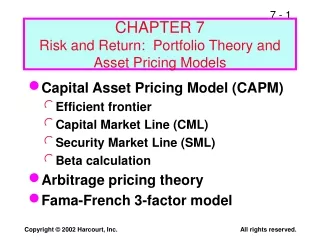
Risk, Return and Portfolio Theory • Risk and risk aversion • Utility theory and the definition of risk aversion • Mean-Variance (M-V or μ-σ) criterion • The mathematics of portfolio theory • Capital allocation and the optimal portfolio • One risky asset and one risk-free asset • Two risky assets • n risky assets • n risky assets and one risk-free asset • Equilibrium in capital markets • The Capital Asset Pricing Model (CAPM) • Market Efficiency
Reward and Risk: Assumptions • Investors prefer more money (reward) to less: all else equal, investors prefer a higher reward to a lower one. • Investors are risk averse: all else equal, investors dislike risk. • There is a tradeoff between reward and risk: Investors will take risks only if they are compensated by a higher reward.
Reward and Risk ☺ Reward ☺ Risk
Quantifying Rewards and Risks • Reward • A welfare measure • The expected (average) return • Risk • A welfare measure • Measures of dispersion - variance • Other measures The mathematics of portfolio theory (1-3)
Comparing Investments:an example Which investment will you prefer and why? • A or B? • B or C? • C or D? • C or E? • D or E? • B or E, C or F? • E or F?
Comparing Investments:the criteria • A vs. B – If the return is certain look for the higher return (reward) • B vs. C – A certain dollar is always better than a lottery with an expected return of one dollar • C vs. D – If the expected return (reward) is the same look for the lower variance of the return (risk) • C vs. E – If the variance of the return (risk) is the same look for the higher expected return (reward) • D vs. E – Chose the investment with the lower variance of return (risk) and higher expected return (reward) • B vs. E or C vs. F – stochastic dominance • E vs. F – maximum expected utility
Comparing Investments Maximum return If the return is risk-free (certain), all investors prefer the higher return Risk aversion Investors prefer a certain dollar to a lottery with an expected return of one dollar
Comparing Investments Maximum expected return If two risky assets have the same variance of the returns, risk-averse investors prefer the one with the higher expected return* Minimum variance of the return If two risky assets have the same expected return, risk-averse investors prefer the one with the lower variance of return*
The Mean-Variance Criterion Let A and B be two (risky) assets. All risk-averse investors prefer asset A to B if { μA ≥ μB and σA < σB } or if { μA > μB and σA ≤ σB } * Note that these rules apply only when we assume that the distribution of returns is normal.
The Utility of Certain Returnsfor Risk Averse Investors Let us assume that the investor has an initial wealth of W0 dollars. Then U(W0) < U(W0 + $1) The utility is an increasing function of the final dollar wealth. U(W0+$1) - U(W0) > U(W0+$101) - U(W0+$100) The utility function is concave: the marginal utility is a decreasing function of the initial dollar wealth (an additional dollar has the same impact on the wealth of the “rich” investor, but it has a lower impact on the his welfare compared to the “poor” investor).
Risk-Averse Investors:Increasing and Concave Utility Function U(W) W
The Expected Utilityof Risky Returns Let DA be the dollar return of asset A (a random variable), DA(i) be the dollar return of asset A in state i (i = 1, … n) and pi be the probability of state i. If you invest in A Your expected dollar wealth is E[W0+DA] = [W0+DA(1)]·p1 + … + [W0+DA(n)]·pn Your expected utility (welfare) is E[U(W0+DA)] = U[W0+DA(1)]·p1 + … + U[W0+DA(n)]·pn
Example (BKM page 193) Consider a simple prospect where all your wealth of $100,000 is invested in a fair gamble: you will get $150,000 with probability 0.5 or $50,000 with probability 0.5. Note that this is called a fair gamble since the expected profit is zero: E(profit) = (150,000-100,000)·0.5 + (50,000-100,000) ·0.5 = 0.
Example - continued • Calculate the expected final wealth. ($100,000) • Assuming that your utility function is logarithmic (i.e. U(W) = ln(W)), calculate your utility of the final wealth for each possible outcome. (11.9184, 10.8198) • Show that for this function the marginal utility is decreasing in the final wealth (numeric example). • Calculate the expected utility of the final wealth and compare it to the utility of the initial wealth. Will you enter the game? (f: 11.3691, i: 11.5129) • How much will you pay me for the right to enter this game? Or should I pay you? ($13,397.5)
The Certainty Equivalent The certainty equivalent (CE) determines the maximum dollar price an investor will pay for a risky asset with an uncertain dollar return D. The expected utility of the investment in the risky asset is equal to that of the certainty equivalent. In our example: E[U(W0+D)] = 0.5·U($50K) + 0.5·U($150K) = 11.3691 11.3691 = U[CE] CE = $86,602.5 That means that you will not invest more than $86,602.5 in that game, or that you will enter the game only if I will pay you a risk premium: $100,000 - $86,602.5 = $13,397.5
Example - continued Assume that you invest $100,000 today (t = 0) and the outcome is expected a year from now (t = 1). What is the present value of the expected future CF if the risk-free rate is 5%? ($82,478.6) What is your personal risk-premium in terms of the dollar difference between a certain CF at time t = 1 and the expected CF of this investment at t = 1? ($13,397.5) What is your personal risk-premium in terms of the required rate of return? (k = 21.24%, k-rf = 16.24%)
Other Criteria The basic intuition is that we care about “bad” surprises rather than all surprises. In fact dispersion (variance) may be desirable if it means that we may encounter a “good” surprise. When we assume that returns are normally distributed the expected-utility and the stochastic-dominance criteria result in the same ranking of investments as the mean-variance criterion.
Practice problems BKM Ch. 6: 1,13,14 BKM Ch. 6, Appendix B: 1 Mathematics of Portfolio Theory: Read and practice parts 1-10.