Download
1 / 124
1.29k likes | 1.33k Views
Data structure. The logical and mathematical model of a particular organization of data is called Data structure . The main characteristics of a data structure are: Contains component data items which may be atomic or another data structure

E N D
The logical and mathematical model of a particular organization of data is called Data structure. The main characteristics of a data structure are: • Contains component data items which may be atomic or another data structure • A set of operations on one or more of the component items • Defines rules as to how components relate to each other and to the structure as a whole The choice of a particular data structure depends on following consideration: • It must be rich enough in structure to mirror actual relationships of data in real world for example the hierarchical relationship of the entities is best described by the “tree” data structure. • The structure should be simple enough that one can effectively process the data when necessary.
The various data structures are divided into following categories: • Linear data structure- A data structure whose elements form a sequence, and every element in structure has a unique predecessor and a unique successor. Examples of linear data structure are: • Arrays • Linked Lists • Stacks • Queues • Non-Linear data structures- A data structure whose elements do not form a sequence. There is no unique predecessor or unique successor. Examples of non linear data structures are trees and graphs.
Linear Data Structures • Arrays- An array is a list of finite number of elements of same data type. The individual elements of an array are accessed using an index or indices to the array. Depending on number of indices required to access an individual element of an array, array can be classified as: • One-dimensional array or linear array that requires only one index to access an individual element of an array • Two dimensional array that requires two indices to access an individual element of array • The arrays for which we need two or more indices are known as multidimensional array.
Linked List- • Linear collection of data elements called nodes • Each node consists of two parts; data part and pointer or link part • Nodes are connected by pointer links. • The whole list is accessed via a pointer to the first node of the list • Subsequent nodes are accessed via the link-pointer member of the current node • Link pointer in the last node is set to null to mark the list’s end • Use a linked list instead of an array when • You have an unpredictable number of data elements (dynamic memory allocation possible) • Your list needs to be sorted quickly
Data member and pointer NULL pointer (points to nothing) 10 15 • Diagram of two data nodes linked together struct node { int data; struct node *nextPtr;} • nextPtr • Points to an object of type node • Referred to as a link • Ties one node to another node
Types of linked lists: • Singly linked list • Begins with a pointer to the first node • Terminates with a null pointer • Only traversed in one direction • Circular, singly linked • Pointer in the last node points back to the first node • Doubly linked list • Two “start pointers” – first element and last element • Each node has a forward pointer and a backward pointer • Allows traversals both forwards and backwards • Circular, doubly linked list • Forward pointer of the last node points to the first node and backward pointer of the first node points to the last node • Header Linked List • Linked list contains a header node that contains information regarding complete linked list.
Stacks-A stack, also called last-in-first-out (LIFO) system, is a linear list in which insertions (push operation) and deletions (pop operations) can take place only at one end, called the top of stack . • Similar to a pile of dishes • Bottom of stack indicated by a link member to NULL • Constrained version of a linked list • The two operations on stack are: push • Adds a new node to the top of the stack pop • Removes a node from the top • Stores the popped value • Returns true if pop was successful
Queues- A queue, also called a First-in-First-out (FIFO) system, is a linear list in which insertions can take place at one end of the list, called the rear of the list and deletions can take place only from other end , called the front of the list. • Similar to a supermarket checkout line • Insert and remove operations
Tree- A tree is a non-linear data structure that represents a hierarchical relationship between various elements. The top node of a tree is called the root node and each subsequent node is called the child node of the root. Each node can have one or more than one child nodes. A tree that can have any number of child nodes is called a general tree. If there is an maximum number N of successors for a node in a tree, then the tree is called an N-ary tree. In particular a binary (2-ary) tree is a tree in which each node has either 0, 1, or 2 successors. • Binary trees • Binary tree can be empty without any node whereas a general tree cannot be empty. • All nodes contain two links • None, one, or both of which may be NULL • The root node is the first node in a tree. • Each link in the root node refers to a child • A node with no children is called a leaf node
47 25 77 11 43 65 93 7 17 31 44 68 • Binary search tree • A type of binary treee • Values in left subtree less than parent • Values in right subtree greater than parent • Facilitates duplicate elimination • Fast searches, maximum of log n comparisons
Graph- A graph, G , is an ordered set (V,E) where V represent set of elements called nodes or vertices in graph terminology and E represent the edges between these elements. This data structure is used to represent relationship between pairs of elements which are not necessarily hierarchical in nature. Usually there is no distinguished `first' or `last' nodes. Graph may or may not have cycles
Algorithms • A finite set of steps that specify a sequence of operations to be carried out in order to solve a specific problem is called an algorithm Properties of Algorithms: 1. Finiteness- Algorithm must terminate in finite number of steps 2. Absence of Ambiguity-Each step must be clear and unambiguous 3. Feasibility-Each step must be simple enough that it can be easily translated into the required language 4. Input-These are zero or more values which are externally supplied to the algorithm 5. Output-At least one value is produced
Conventions Used for Algorithms • Identifying number-Each algorithm is assigned as identification number • Comments-Each step may contain a comment in brackets which indicate the main purpose of the step • Assignment statement-Assignment statement will use colon-equal notation • Set max:= DATA[1] • Input/Output- Data may be input from user by means of a read statement • Read: Variable names • Similarly, messages placed in quotation marks, and data in variables may be output by means of a write statement: • Write: messages or variable names
Selection Logic or conditional flow- • If condition, then: • [end of if structure] • Double alternative • If condition, then • Else: • [End of if structure] • Multiple Alternatives • If condition, then: • Else if condition2, then: • Else if condition3, then • Else: • [End of if structure]
Iteration Logic • Repeat- for loop • Repeat for k=r to s by t: • [End of Loop] • Repeat-While Loop • Repeat while condition: • [End of loop]
Algorithm complexity • An algorithm is a sequence of steps to solve a problem. There can be more than one algorithm to solve a particular problem and some of these solutions may be more efficient than others. The efficiency of an algorithm is determined in terms of utilization of two resources, time of execution and memory. This efficiency analysis of an algorithm is called complexity analysis, and it is a very important and widely-studied subject in computer science. Performance requirements are usually more critical than memory requirements. Thus in general, the algorithms are analyzed on the basis of performance requirements i.e running time efficiency. • Specifically complexity analysis is used in determining how resource requirements of an algorithm grow in relation to the size of input. The input can be any type of data. The analyst has to decide which property of the input should be measured; the best choice is the property that most significantly affects the efficiency-factor we are trying to analyze. Most commonly, we measure one of the following : • the number of additions, multiplications etc. (for numerical algorithms). • the number of comparisons (for searching, sorting) • the number of data moves (assignment statements) .
Based on the type of resource variation studied, there are two types of complexities • Time complexity • Space complexity Space Complexity- The space complexity of an algorithm is amount of memory it needs to run to completion. The space needed by a program consists of following components: • Instruction space-space needed to store the executable version of program and is fixed. • Data space-space needed to store all constants, variable values and has further two components: • Space required by constants and simple variables. This space is fixed. • Space needed by fixed sized structured variable such as arrays and structures. • Dynamically allocated space. This space usually varies.
Environment stack space- Space needed to store information needed to resume the suspended functions. Each time a function is invoked following information is saved on environment stack • Return address i.e from where it has to resume after completion of the called function • Values of all local variables and values of formal parameters in function being invoked. Time complexity- Time complexity of an algorithm is amount of time it needs to run to completion. To measure time complexity, key operations are identified in a program and are counted till program completes its execution. Time taken for various key operations are: • Execution of one of the following operations takes time 1: 1. assignment operation 2. single I/O operations 3. single Boolean operations, numeric comparisons 4. single arithmetic operations 5. function return 6. array index operations, pointer dereferences
Running time of a selection statement (if, switch) is the time for the condition evaluation + the maximum of the running times for the individual clauses in the selection. • Loop execution time is the number of times the loop body is executed + time for the loop check and update operations, + time for the loop setup. † Always assume that the loop executes the maximum number of iterations possible • Running time of a function call is 1 for setup + the time for any parameter calculations + the time required for the execution of the function body.
Expressing Space and time complexity: Big ‘O’ notation • It is very difficult to practically analyze the variation of time requirements of an algorithm with variation in size of input. A better approach to express space/time complexity is in the form of a function f (n) where n is the input size for a given instance of problem being solved. Efficiency (algorithm A) = a function F of some property of A's input. • We have to decide which property of the input we are going to measure; the best choice is the property that most significantly affects the efficiency-factor we are trying to analyze. For example, the time taken to sort a list is invariably a function of the length of the list. The speed of an algorithm varies with the number of items n. • The most important notation used for expressing this function f(n) is Big O notation.
Big O notation is a characterization scheme that allows to measure the properties of algorithm such as performance and/or memory requirements in general fashion. big ‘O’ notation • Uses the dominant term of the function • Omits lower order terms and coefficient of dominant Apart from n (size of input), efficiency measure will depend on three cases which will decide number of operations to be performed. • Best- Case performance under ideal condition • Worst-case performance under most un favorable condition • Average case performance under most probable condition. Big ‘O’ notation tries to analyze each algorithm performance in worst condition. It is the rate of increase of f(n) that is examined as a measure of efficiency.
Rate of growth: Big O notation • Suppose F is an algorithm and suppose n is the size of input data. Clearly, complexity f(n) of F increases as n increases. Rate of increase of f(n) is examined by comparing f(n) with some standard functions such as log2n, n, nlog2n, n2,n3 and 2n. One way to compare f(n) with these standard functions is to use functional O notation defined as follows: • Definition: If f(n) and g(n) are functions defined on positive integers with the property that f(n) is bounded by some multiple of g(n) for almost all n. That is, suppose there exist a positive integer no and a positive number M such that for all n> no we have |f(n) | ≤ M |g(n)| • Then we may write f(n)=O g(n) Which is read as f(n)(time taken for number of operations) is of the order of g(n). If g(n)=n, it means that f(n) is a linear proportional to n. For g(n)=n2 , f(n) is proportional to n2. Thus if an array is being sorted using an algorithm with g(n)=n2, it will take 100 times as long to sort the array that is 10 times the size of another array.
Based on Big O notation, algorithms can be categorized as • Constant time ( O(1)) algorithms • Logarithmic time algorithms (O(logn)) • Linear Time algorithm (O(n) • Polynomial or quadratic time algorithm (O(nk)) • Exponential time Algorithm (O(kn)) • It can be seen that logarithmic function log(n) grows most slowly whereas kn grows most rapidly and polynomial function nk grows in between the two extremities. Big-O notation, concerns only the dominant term, low-order terms and constant coefficients are ignored in a statement. Thus if g(n) = n2+2n, the variation is taken as O(n2) rather than O(n). Complexities of some well known searching and sorting algorithms is: • Linear Search: O(n) Mergesort: O(nlogn) • Binary Search: O(logn) • Bubble sort: O(n2)
RUNNING TIME • let f(n) be the function that defines the time an algorithm takes for problem size n. The exact formula for f(n) is often difficult to get. We just need an approximation • What kind of function is f ? • Is it constant? linear? quadratic? .... and, our main concern is large n. Other factors may dominate for small n
COMPLEXITY SAMPLES • assume different algorithms to solve a problem • with time functions:T1(n), T2(n), T3(n), T4(n) • plot each for a range of n
2n 108 n3 107 Time taken n2 106 105 nlogn 104 n 103 logn 102 1 100 1000 10 10,000 Input size n Rate of Growth of f(n) with n
Other Asymptotic notations for Complexity Analysis The big ‘O’ notation defines the upper bound function g(n) for f(n) which represents the time/space complexity of the algorithm on an input characteristic n . The other such notations are: • Omega Notation (Ω)- used when function g(n) defines the lower bound for function f(n). It is defined as |f(n)| ≥ M|g(n)| • Theta Notation (Θ)- Used when function f(n) is bounded both from above and below by the function g(n). It is defined as c1|g(n)| ≤ |f(n)| ≤ c2.|g(n)| Where c1 and c2 are two constants. • Little oh Notation (o)- According to this notation, f(n)=o g(n) iff f(n) = Og(n) and f(n)≠ Ωg(n)
Time-Space Tradeoff- The best algorithm to solve a given problem is one that requires less space in memory and takes less time to complete its execution. But in practice, it is not always possible to achieve both of these objectives. Thus, we may have to sacrifice one at the cost of other. This is known as Time-space tradeoff among algorithms. Thus if space is our constraint, we have to choose an algorithm that requires less space at the cost of more execution time. On the other hand, if time is our constraint, such as in real time systems, we have to choose a program that takes less time to complete execution at the cost of more space.
Various operations performed on Arrays • Traversal- processing each element in the list • Searching- Finding location of an element • Insertion- Adding a new element • Deletion- Removing an element • Sorting-Arranging elements in some type of order • Merging- Combining two lists into a single list
Traversing Linear Arrays- Traversing a linear array is basically, visiting each element of array exactly once. Traversing is usually required to count number of elements of array or to perform other operations on each element of array. Traversing a linear array depends on size of array. Thus, traversal is O(n) operation for an array of size n. • Algorithm: (Traversing a linear Array) Here LA is a linear array with lower bound LB and upper Bound UB. This algorithm traverses LA applying an operation PROCESS to each element of LA • Step 1: [Initialize Counter] Set k:=LB • Step 2: Repeat step 3 and 4 while k<=UB Repeat for k=LB to UB: • Step 3: [Visit Element] Apply PROCESS Apply PROCESS to • to LA[k] LA[k] • Step 4: [increase Counter] set k:=k+1 • [End of step 2 loop] • Step 5: Exit
Insertion and Deletion in an Array- Insertion refers to operation of adding an element to an array and deletion refers to deleting an element from an array • Insertion- Insertion can be done at various positions but the main cases undertaken are: • Insertion at the start • Insertion at the end • Insertion in the middle • Insertion at any other position Inserting an element at the end of the array can be done easily provided the memory space allocated for the array is large enough to accommodate the additional element. For inserting at any other position, elements of array have to be shifted downwards from the position where insertion is to be done. The new element is then inserted in vacated position.
Algorithm: (Inserting into a Linear Array) INSERT(LA,N,K,ITEM) Here LA is a linear array with N elements and K is a positive integer such that K<=N. This algorithm inserts an element ITEM into Kth position in LA. • Step 1: [Initialize counter] Set J:=N • Step 2: Repeat steps 3 and 4 while J ≥ K: [Move Jth element downward] Set LA[J+1]:=LA[J] [ Decrease Counter] Set J:=J -1 [End of Step 2 Loop] • Step 3: [Insert element] Set LA[K]:=ITEM • Step 4:[Reset N] Set N:=N+1 • Step 5: Return
Deletion refers to the operation of removing an element from exiting list of elements. Like insertion, deletion can be done easily from the end of the list. However to delete an element from any other location, the elements are to be moved upwards in order to fill up the location vacated by the removed element.
Algorithm: (Deleting from a Linear Array) DELETE(LA,N,K,ITEM) Here LA is a linear array with N elements and K is a positive integer such that K<=N. This algorithm deletes an element ITEM from Kth position in LA. • Step 1: [Initialize counter] Set ITEM:=LA[K] • Step 2: Repeat for J=K to N-1: [Move J+1st element upward] Set LA[J]:=LA[J+1] [End of Step 2 Loop] • Step 3: [Reset N] Set N:=N+1 • Step 4: Return
Analysis of Insertion and deletion operation • The best possible case in insertion operation is when the item is inserted at the last position. In this case, no movement of elements is required. The worst case occurs when the element has to be inserted at the beginning of the list. In this case, we have to move all the elements down the list. Therefore, the while loop executes n times, each moving one element down. Thus complexity of insertion operation is O(n), i.e linear time. • The best case in deletion occurs when the element to be deleted is the last element of the array. In this case, no element is moved up. The worst case occurs when element is deleted from the first position. In this case, all (n-1) elements are moved up. The while loop executes n-1 times, each time moving one element down. Thus complexity of deletion operation is also O(n) i.e linear time.
Algorithm: (Linear Search) LINEAR(DATA, N, ITEM, LOC) Here DATA is a linear array with N elements and ITEM is a given item of information. This algorithm finds the location LOC of ITEM in DATA, or sets LOC:=0 if search is unsuccessful. • Step 1: [Initialize Counter] Set LOC:=1 • Step 2: [Search for ITEM] Repeat while LOC<=N: If DATA[LOC] = ITEM, Then: Write: ’Element is at the location’, LOC Exit [End of if structure] Set LOC:=LOC+1 [End of Loop] • Step 3: [Unsuccessful] If LOC=N+1 , then: Set LOC:=0 • Step 4: Return
Binary Search: Binary search is a method of searching in which array list is divided into two equal parts. The main requirement of binary search method is that the array has to be in sorted order. If the elements of array list are in ascending order, then , if desired element is less than the middle element of the list, it will never be present in second half of the array and if desired element is greater than middle element, it will never be present in first half of the array list. Thus focus is given only to the desired half of the array list. • Algorithm: BINARY(DATA, LB, UB, ITEM, LOC) Here DATA is a sorted array with lower bound LB and upper bound UB, and the ITEM is a given item of information. The variables BEG, END and MID denote, beginning, end and middle location of a segment of elements of DATA. This algorithm finds the location LOC of ITEM in DATA or set LOC=NULL • Step 1: [Initialize segment variable] Set BEG:=LB, END:=UB and MID:= INT((BEG+END)/2)
Step 2: Repeat while BEG<=END and DATA[MID]≠ITEM If ITEM < DATA[MID], then: Set END:= MID -1 Else: Set BEG:= MID +1 [End of if structure] • Step 3: Set MID:=INT((BEG+END)/2) [End of step2 loop] • Step 4: If DATA[MID]=ITEM, then: Set LOC:=MID Else : Set LOC:=NULL [End of if structure] • Step 5: Return
Analysis of Linear Search and Binary Search • LINEAR SEARCH • In best possible case, item may occur at first position. In this case, search operation terminates in success with just one comparison. However, the worst case occurs when either item is present at last position or element is not there in the array. In former case, search terminates in success with n comparisons. In latter case, search terminates in failure with n comparisons. Thus in worst case, the linear search is O(n) operation. In average case, the average number of comparisons required o find the location of item is approximately equal to half of the number of elements in the array. • BINARY SEARCH • In each iteration or in each recursive call, search is reduced to one half of the size of array. Therefore, for n elements, there will be log2n iterations or recursive calls. Thus complexity of binary search is O(log2n). This complexity will be same irrespective of position of element, even if it is not present in array.
Sorting Techniques in Array • Bubble sort method- The bubble sort method requires n-1 passes to sort an array where n is the size of array. In each pass, every element of the array a[i] is compared with a[i+1] for i=0 to n-k where k is the pass number. If a[i]>a[i+1], they are swapped. This will cause largest element to move or bubble up.
Algorithm: BUBBLE(DATA, N) Here DATA is an array with N elements. This algorithm sorts the elements in DATA. • Step 1: Repeat step 2 and 3 for K=1 to N-1: • Step 2: [Initialize pass pointer PTR] Set PTR:=1 • Step 3:[Execute Pass] Repeat while PTR ≤ N-K • IF DATA[PTR] > DATA[PTR + 1], then: Interchange DATA[PTR] and DATA[PTR + 1] [End of If structure] Set PTR:=PTR +1 [End of Step 3 loop] [End of Step 1 Loop] • Step 4: Return
Complexity analysis of Bubble sort method: Traditionally, time for sorting an array is measured in terms of number of comparisons. The number f(n) of comparisons in bubble sort is easily computed. Specifically, there are n-1 comparisons during first pass, n-2 comparisons in second pass and so on. Thus, f(n)=(n-1) +(n-2) +-------+2+1 = n(n-1)/2 = n2 / 2 – n/2 = O(n2) Thus time required to sort an array using bubble sort method is proportional to n2 where n is number of input items. Thus complexity of bubble sort is O(n2)