Download
1 / 41
420 likes | 769 Views
Animation in Video Games. presented by Jason Gregory. jgregory@ea.com. Agenda. The Goal of Game Animation Old School Animation Skeletons and Skins How Skinning Works (Graphically) The Math of Skinning Animation: Bringing a Character to Life Blending and other Advanced Topics.

E N D
Animation in Video Games presented by Jason Gregory jgregory@ea.com
Agenda • The Goal of Game Animation • Old School Animation • Skeletons and Skins • How Skinning Works (Graphically) • The Math of Skinning • Animation: Bringing a Character to Life • Blending and other Advanced Topics
The Goal of Game Animation • Our goal is simple: To produce realistic looking animated characters in our games!
Old School Animation • The very first animated characters were 2D sprites. • Just like traditional cel animation or flip books.
Old School Animation (3) • When we moved to 3D, our first animated characters were “jointed.” • Each limb or part of a limb is a separate rigid object. • Problem: Interpenetration at joints!
Skeletons and Skins • Modern approach is called “skinning.” • Basic idea: • Create a jointed skeleton. • Attach the skin to the skeleton. • Move skeleton around – skin follows it. • Skin is a 3D model made out of triangles. • Skeleton is invisible – only the skin is seen by the player.
Skeletons and Skins (3) • Each vertex of each triangle is attached to one or more bones. • We use weights to define bones’ influences. • Weights at a joint must always add up to 1.
Skeletons and Skins (5) • Skeletons have two kinds of poses: • Bind Pose: The skeleton’s pose when the skin was first attached. • Current Pose: Any other pose of the skeleton; usually a frame of an animation. • The bind pose is like a “home base” for the character’s skeleton. • If you drew the mesh without its skeleton, it would appear in its bind pose.
Skeletons and Skins (6) Bind Pose Current Pose
How Skinning Works • Consider a single vertex (v) skinned to the joint J1. The skeleton is in bind pose: v y J1 J0 x
How Skinning Works (2) • We want to find the vertex’s new location (v') in the current pose. v y v' x
How Skinning Works (3) • The basic idea is to transform the vertex: • from model space • into joint space • The coordinates of the vertex are invariant in joint space! • So, we can move the joint around all we want. • When we’re done, we go back to model space to find the final position (v').
How Skinning Works (4) • Here’s the original vertex (v), but now in the joint space of J1: v y J1 J0 x
How Skinning Works (5) • No matter what pose the skeleton is in, v and v' are the same when in joint space. v y v' x
How Skinning Works (6) • Finally, we go back to model space to find the final location of the vertex (v'). v y v' x
The Math of Skinning • Let Xi be the translation of joint i. v y X1 X0 x
The Math of Skinning (2) • Let Qi be the rotation of joint i. v y Q1 Q0 x
The Math of Skinning (3) • We describe the bind posematrix of joint J1 as the matrix product of all the translations and rotations from the root joint to the joint in question:
The Math of Skinning (4) • Now consider what happens when we move the skeleton into the current pose: y v' J0 J1 x
The Math of Skinning (5) • This time, let Ti be the translation of joint i,and let Ri be the rotation of joint i: y R0 v' T0 R1 T1 x
The Math of Skinning (6) • The matrix describing the current pose is: which is similar to the bind pose matrix:
The Math of Skinning (7) • We multiply v by B–1 to get it into joint space from the bind pose. • Then we multiply that by Pto get it back into model space, in the current pose.
The Math of Skinning (8) • Mathematically, this is:
The Math of Skinning (9) • Voila! We can find v' for any pose imaginable! v y v' x
The Math of Skinning (10) • We do these calculations on each and every vertex in the model. • Then we draw the final vertices. • For vertices that are affected by more than one joint, we take a weighted average of the positions due to each joint.
The Math of Skinning (11) • The weighted average for a vertex affected by joints j and k would be:
Animation: Bringing Characters to Life • An animation is really just a sequence of poses at various points in time. The poses are called keys. • An animation can be described mathematically as: { Pj (t) } ji.e. a set of pose matrices (keys) for all joints j, each of which is a function of time t. • To play back the animation, we extract a pose at the current time index, skin the model to that pose, and then draw the model.
Bringing Characters to Life (2) • Run Weasel, run!
Bringing Characters to Life (3) • In a simple animation system, the keys are equally spaced in time. • If we further restrict ourselves to integer time indices, then extracting a pose amounts to selecting the appropriate key. Joint 1: Joint 2: Joint 3: … N–1 time 0 1 2 3 4 … time = t
Bringing Characters to Life (3) • To reduce memory overhead, the keys can be compressed, and might not be uniformly spaced. • We will want to allow the time index to be a real number (i.e. floating-point). • So, extracting a pose now requires interpolation between adjacent key frames. Joint 1: Joint 2: Joint 3: … N–1 time 0 1 2 3 4 … time = t
Interpolation and Blending • To interpolate positions, we use simple vector linear interpolation (LERP).
Interpolation and Blending (2) • To interpolate rotations, we must use quaternions. (It is next to impossible to interpolate matrices.) • We have two choices when interpolating quats: • Linear interpolation (LERP) • Spherical linear interpolation (SLERP)
Interpolation and Blending (3) • A quaternion LERP is identical to a vector LERP, but with 4 components. • SLERP is like a LERP, but the weights are no longer (1-) and . Instead they are:
Interpolation and Blending (4) • LERP and SLERP can be used to interpolate between adjacent key frames for a specific time t. • Interpolation can also be used to blend two entirely different animations together! • For example, instead of a character being able to walk or run, he can do anything in between! • The blend factor controls how much walk and how much run we see. =0: full walk =1: full run=0.5: half walk, half run
The Animation Pipeline • Typical animation pipeline: • Pose extraction at current time t • Pose blending • Matrix palette generation • Palette-driven rendering • The matrix palette maps directly to modern vertex shader architectures (a.k.a. indexed skinning).
Advanced Topics • Key frame compression techniques • Representing animations as spline curves instead of interpolated key frames • Action state machines • Skeletal partitioning • Rag-doll physics • …
Q&A • Thanks for your attention! • Questions can also be sent to: Jason GregoryElectronic Arts Los Angelesjgregory@ea.com