Download
1 / 85
850 likes | 1.05k Views
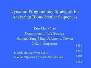
Dynamic Programming Method for Analyzing Biomolecular Sequences. Tao Jiang Department of Computer Science University of California - Riverside (Typeset by Kun-Mao Chao) E-mail: jiang@cs.ucr.edu http://www.cs.ucr.edu/~jiang. Outline. The paradigm of dynamic programming

E N D
Dynamic Programming Method for Analyzing Biomolecular Sequences Tao Jiang Department of Computer Science University of California - Riverside (Typeset by Kun-Mao Chao) E-mail: jiang@cs.ucr.edu http://www.cs.ucr.edu/~jiang
Outline • The paradigm of dynamic programming • Sequence alignment – a general framework for comparing sequences in bioinformatics • Dynamic programming algorithms for sequence alignment • Techniques for improving the efficiency of the algorithms • Multiple sequence alignment
Dynamic Programming • Dynamic programming is an algorithmic method for solving optimization problems with a compositional/recursive cost structure. • Richard Bellman was one of the principal founders of this approach.
Two key features • Two key features of an optimization problem to be suitable for a dynamic programming solution: 1. optimal substructures 2. overlapping subinstances Subinstances are dependent. (Otherwise, a divide-and-conquer approach is the choice.) Each substructure is optimal. (principle of optimality)
Three basic components • The development of a dynamic programming algorithm has three basic components: • A recurrence relation (for defining the value/cost of an optimal solution); • A tabular computation (for computing the value of an optimal solution); • A backtracing procedure (for delivering an optimal solution).
= F 0 0 = F 1 1 = + F F F for i>1 . - - i i 1 i 2 Fibonacci numbers The Fibonacci numbers are defined by the following recurrence:
F8 F9 F7 F10 F7 F8 F6 How to compute F10? ……
Tabular computation • Tabular computation can avoid redundant computation steps.
Maximum sum interval • Given a sequence of real numbers a1a2…an, find a consecutive subsequence with the maximum sum. 9 –3 1 7 –15 2 3 –4 2 –7 6 –2 8 4 -9 For each position, we can compute the maximum-sum interval starting at that position in O(n) time. Therefore, a naive algorithm runs in O(n2) time.
cg(n) f(n) n0 O-notation:an asymptotic upper bound • f(n) = O(g(n)) iff there exist two positive constant c and n0 such that 0 f(n) cg(n) for all n n0 For example, 5n + 108 = O(n) and 2n = O(nlog n).
How functions grow? function For large data sets, algorithms with a complexity greater than O(n log n) are often impractical! n (Assume one million operations per second.)
ai Maximum sum interval(the recurrence relation) • Define S(i) to be the maximum sum of the intervals ending at position i. If S(i-1) < 0, concatenating ai with its previous interval gives less sum than ai itself.
Maximum sum interval(tabular computation) 9 –3 1 7 –15 2 3 –4 2 –7 6 –2 8 4 -9 S(i) 9 6 7 14 –1 2 5 1 3 –4 6 4 12 16 7 The maximum sum
Maximum sum interval(backtracing) 9 –3 1 7 –15 2 3 –4 2 –7 6 –2 8 4 -9 S(i) 9 6 7 14 –1 2 5 1 3 –4 6 4 12 16 7 The maximum-sum interval: 6 -2 8 4 Running time: O(n).
Two fundamental problems we solved (joint work with Lin and Chao) • Given a sequence of real numbers of length n and an upper bound U, find a consecutive subsequence of length at most U with the maximum sum --- an O(n)-time algorithm. U = 3 9 –3 1 7 –15 2 3 –4 2 –7 6 –2 8 4 -9
Two fundamental problems we solved (joint work with Lin and Chao) • Given a sequence of real numbers of length n and a lower bound L, find a consecutive subsequence of length at least L with the maximum average --- an O(n log L)-time algorithm. This was improved to O(n) by others later. L = 4 3 2 14 6 6 2 10 2 6 6 14 2 1
Another example Given a sequence as follows: 2, 6.6, 6.6, 3, 7, 6, 7, 2 and L = 2, the highest-average interval is the squared area, which has the average value 20/3. 2, 6.6, 6.6, 3, 7, 6, 7, 2
GC-rich regions • Our method can be used to locate a region of length at least L with the highest C+G ratio in O(n log L) time. ATGACTCGAGCTCGTCA 00101011011011010 Search for an interval of length at least L with the highest average.
Length-unconstrained version • Maximum average interval 3 2 14 6 6 2 10 2 6 6 14 2 1 The maximum element is the answer. It can be done in O(n) time.
A naive algorithm • A simple shift algorithm can compute the highest-average interval of a fixed length in O(n) time • Try L, L+1, L+2, ..., n. In total, O(n2).
A pigeonhole principle • Notice that the length of an optimal interval is bounded by 2L, we immediately have an O(nL)-time algorithm. We can bisect a region of length >= 2L into two segments, where each of them is of length >= L.
Longest increasing subsequence (LIS) • The longest increasing subsequence problem is to find a longest increasing subsequence of a given sequence of integers a1a2…an. e.g. 9 2 5 3 7 11 8 10 13 6 • 3 7 • 7 10 13 • 7 11 3 5 11 13 are increasing subsequences. We want to find a longest one. are not increasing subsequences.
A standard DP approach for LIS • Let L[i] be the length of a longest increasing subsequence ending at position i. L[i] = 1 + max j = 0..i-1{L[j] | aj < ai}(use a dummy a0 = maximum, and L[0]=0) 9 2 5 3 7 11 8 10 13 6 L[i] 1 1 2 2 3 4 ?
A standard DP approach for LIS L[i] = 1 + max j = 0..i-1{L[j] | aj < ai} 9 2 5 3 7 11 8 10 13 6 L[i] 1 1 2 2 3 4 4 5 6 3 The maximum length The subsequence 2, 3, 7, 8, 10, 13 is a longest increasing subsequence. This method runs in O(n2) time.
Binary Search • Given an ordered sequence x1x2 ... xn, where x1<x2< ... <xn, and a number y, a binary search finds the largest xi such that xi< y in O(log n) time. n/2 ... n/4 n
Binary Search • How many steps would a binary search reduce the problem size to 1?n n/2 n/4 n/8 n/16 ... 1 How many steps? O(log n) steps.
An O(n log n) method for LIS • Define BestEnd[k] to be the smallest end number of an increasing subsequence of length k. 9 2 5 3 7 11 8 10 13 6 9 2 2 2 2 2 2 2 2 BestEnd[1] 5 3 3 3 3 3 3 BestEnd[2] 7 7 7 7 7 BestEnd[3] 11 8 8 8 BestEnd[4] 10 10 BestEnd[5] 13 BestEnd[6]
An O(n log n) method for LIS • Define BestEnd[k] to be the smallest end number of an increasing subsequence of length k. 9 2 5 3 7 11 8 10 13 6 9 2 2 2 2 2 2 2 2 2 BestEnd[1] 5 3 3 3 3 3 3 3 BestEnd[2] 7 7 7 7 7 6 BestEnd[3] 11 8 8 8 8 BestEnd[4] For each position, we perform a binary search to update BestEnd. Therefore, the running time is O(n log n). 10 10 10 BestEnd[5] 13 13 BestEnd[6]
Longest Common Subsequence (LCS) • A subsequence of a sequence S is obtained by deleting zero or more symbols from S. For example, the following are all subsequences of “president”: pred, sdn, predent. • The longest common subsequence problem is to find a maximum length common subsequence between two sequences.
LCS For instance, Sequence 1: president Sequence 2: providence Its LCS is priden. president providence
LCS Another example: Sequence 1: algorithm Sequence 2: alignment One of its LCS is algm. a l g o r i t h m a l i g n m e n t
How to compute LCS? • Let A=a1a2…am and B=b1b2…bn . • len(i, j): the length of an LCS between a1a2…ai and b1b2…bj • With proper initializations, len(i, j) can be computed as follows.
Pairwise Alignment Sequence A: CTTAACT Sequence B: CGGATCAT An alignment of A and B: C---TTAACTCGGATCA--T Sequence A Sequence B
Pairwise Alignment Sequence A: CTTAACT Sequence B: CGGATCAT An alignment of A and B: Mismatch Match C---TTAACTCGGATCA--T Deletion gap Insertion gap
Alignment (or Edit) Graph C G G A T C A T Sequence A: CTTAACT Sequence B: CGGATCAT CTTAACT C---TTAACTCGGATCA--T
A simple scoring scheme • Match: +8 (w(x, y) = 8, if x = y) • Mismatch: -5 (w(x, y) = -5, if x ≠ y) • Each gap symbol: -3 (w(-,x)=w(x,-)=-3) (i.e. space) C - - - T T A A C TC G G A T C A - - T +8 -3 -3 -3 +8 -5 +8 -3 -3 +8 = +12 alignment score
Scoring Matrices • Amino acid substitution matrices • PAM • BLOSUM • DNA substitution matrices • DNA is less conserved than protein sequences • Less effective to compare coding regions at nucleotide level
PAM • Point Accepted Mutation (Dayhoff, et al.) • 1 PAM = PAM1 = 1% average change of all amino acid positions • After 100 PAMs of evolution, not every residue will have changed • some residues may have mutated several times • some residues may have returned to their original state • some residues may not have changed at all
PAMX • PAMx = PAM1x E.g. PAM250 = PAM1250 • PAM250 is a widely used scoring matrix. Ala Arg Asn Asp Cys Gln Glu Gly His Ile Leu Lys ... A R N D C Q E G H I L K ... Ala A 13 6 9 9 5 8 9 12 6 8 6 7 ... Arg R 17 4 3 2 5 3 2 6 3 2 9 Asn N 6 7 2 5 6 4 6 3 2 5 Asp D 11 1 7 10 5 6 3 2 5 Cys C 52 1 1 2 2 2 1 1 Gln Q 10 7 3 7 2 3 5 ... Trp W 1 0 1 0 Tyr Y 2 2 1 Val V 15 10
BLOSUM • Blocks Substitution Matrix • Scores derived from observations of the frequencies of substitutions in blocks of local alignments in related proteins • Matrix name indicates evolutionary distance • BLOSUM62 was created using sequences sharing no more than 62% identity
An optimal alignment-- an alignment of maximum score • Let A=a1a2…am and B=b1b2…bn . • Si,j: the score of an optimal alignment between a1a2…ai and b1b2…bj • With proper initializations, Si,j can be computedas follows.
Computing Si,j j w(ai,bj) w(ai,-) i w(-,bj) Sm,n
Initialization C G G A T C A T CTTAACT
S3,5 = ? C G G A T C A T CTTAACT
S3,5 = ? C G G A T C A T CTTAACT optimal score