Download

1 / 51
530 likes | 561 Views
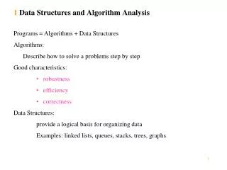
Data Structures and Algorithm Analysis Graph Algorithms. Lecturer: Jing Liu Email: neouma@mail.xidian.edu.cn Homepage: http://see.xidian.edu.cn/faculty/liujing. Definitions. A graph G =( V , E ) consists of a set of vertices , V , and a set of edges , E .

E N D
Data Structures and Algorithm AnalysisGraph Algorithms Lecturer: Jing Liu Email: neouma@mail.xidian.edu.cn Homepage: http://see.xidian.edu.cn/faculty/liujing
Definitions • A graphG=(V, E) consists of a set of vertices, V, and a set of edges, E. • Each edge is a pair (v, w), where v, wV. Edges are sometimes referred to as arcs. If the pair is ordered, then the graph is directed. • Vertex w is adjacent to v if and only if (v, w)E. In an undirected graph with edge {v, w}, w is adjacent to v and v is adjacent to w. Some times an edge has a third component, known as either a weight or a cost.
Definitions • A path in a graph is a sequence of vertices w1, w2, w3, …, wN such that (wi, wi+1)E for 1i<N. The length of such a path is the number of edges on the path, which is equal to N-1. • We allow a path from a vertex to itself; if this path contains no edges, then the path length is 0. • If the graph contains an edge (v, v) from a vertex to itself, then the path v, v is sometime referred to as a loop. The graphs we will consider will generally be loopless. • A simple path is a path such that all vertices are distinct, except that the first and the last could be the same.
Definitions • A cycle in a directed graph is a path of length at least 1 such that w1=wn; this cycle is simple if the path is simple. • For undirected graphs, we require that the edges be distinct; that is, the path u, v, u in an undirected graph should not be considered a cycle, because (u, v) and (v, u) are the same edge. In a directed graph, these are different edges, so it makes sense to call this a cycle. • A directed graph is acyclic if it has no cycles.
Definitions • An undirected graph is connected if there is a path from every vertex to every other vertex. A directed graph with this property is called strongly connected. If a directed graph is not strongly connected, but the underlying graph (without direction to the arcs) is connected, then the graph is said to be weakly connected. • A complete graph is a graph in which there is an edge between every pair of vertices.
Definitions • In an undirected graph, the degree of a vertex is the number of edges connected to this vertex. • In an directed graph, the outdegree of a vertex is the number of edges that start from this vertex, and the indegree is the number of edges that end at this vertex. • Examples of graphs: airport system, traffic flow, friendship.
Representation of Graphs • Suppose, for now, that we can number the vertices, starting at 1; that is, V={1, 2, …, n} • One simple way to represent a graph is to use a two-dimensional array this is known as a adjacency matrix representation. • For each edge (u, v), we set A[u][v]=1; otherwise the entry in the array is 0. • If the edge has a weight associated with it, then we can set A[u][v] equal to the weight and use either a very large or a very small weight as a sentinel to indicate nonexistent edges.
Representation of Graphs • If the number of edges in a graph is very small, a better solution is an adjacency list representation. • For each vertex, we keep a list of all adjacent vertices: The leftmost structure is merely an array of header cells. If the edges have weights, then this additional information is also stored in the cells.
Topological Sort • A topological sort is an ordering of vertices in a directed acyclic graph, such that if there is a path from vi to vj, then vj appears after vi in the ordering. • See Figure 9.3: A directed edge (v, w) indicates that course v must be completed before course w may be attempted. A topological ordering of these courses is any course sequence that does not violate the prerequisite requirement.
Topological Sort • It is clear that a topological ordering is not possible if the graph has a cycle, since for two vertices v and w on the cycle, v precedes w and w precedes v. • The ordering is not necessarily unique; any legal ordering will do. • A simple algorithm to find a topological ordering is first to find any vertex with no incoming edges. We can then print this vertex, and remove it, along with this edge, from the graph. Then we apply this same strategy to the rest of the graph. • Thus, we compute the indegrees of all vertices in the graph, and look for a vertex with indegree 0 that has not already been assigned a topological number.
Example: Topological Sort 1 2 3 4 5 6 7
The All-Pairs Shortest Path Problem • Let G=(V, E) be a directed graph in which each edge (i, j) has a non-negative length l[i, j]. If there is no edge from vertex i to vertex j, then l[i, j]=. • The problem is to find the distance from each vertex to all other vertices, where the distance from vertex x to vertex y is the length of a shortest path from x to y. • For simplicity, we will assume that V={1, 2, …, n}. Let i and j be two different vertices in V. Define to be the length of a shortest path from i to j that does not pass through any vertex in {k+1, k+2, …, n}.
The All-Pairs Shortest Path Problem • is the length of a shortest path from i to j that does not pass through any vertex except possibly vertex 1 • is the length of a shortest path from i to j that does not pass through any vertex except possibly vertex 1 or vertex 2 or both • is the length of a shortest path from i to j, i.e. the distance from i to j
The All-Pairs Shortest Path Problem • We can compute recursively as follows:
The All-Pairs Shortest Path Problem • Floyd Algorithm: use n+1 matrices D0, D1, D2, …, Dn of dimension nn to compute the lengths of the shortest constrained paths. • Initially, we set D0[i, i]=0, D0[i, j]=l[i, j] if ij and (i, j) is an edge in G; otherwise D0[i, j]=. • We then make n iterations such that after the kth iteration, Dk[i, j] contains the value of a shortest length path from vertex i to vertex j that does not pass through any vertex numbered higher than k.
The All-Pairs Shortest Path Problem • Thus, in the kth iteration, we compute Dk[i, j] using the formula Dk[i, j]=min{Dk-1[i, j], Dk-1[i, k]+Dk-1[k, j]}
The All-Pairs Shortest Path Problem • Example: 1 1 2 9 8 3 2 6
The All-Pairs Shortest Path Problem • Input: An nn matrix l[1…n, 1…n] such that l[i, j] is the length of the edge (i, j) in a directed graph G=({1, 2, …, n}, E); • Output: A matrix D with D[i, j]=the distance from i to j; • 1. Dl; • 2. for k1 to n • 3. for i1 to n • 4. for j1 to n • 5. D[i, j]=min{D[i, j], D[i, k]+D[k, j]); • 6. end for; • 7. end for; • 8. end for;
The All-Pairs Shortest Path Problem • What is the time and space complexity of the FLOYD algorithm?
The All-Pairs Shortest Path Problem • The running time of FLOYD algorithm is (n3) and its space complexity is (n2).
The Shortest Path Problem • Let G=(V, E) be a directed graph in which each edge has a nonnegative length, and a distinguished vertex s called the source. The single-source shortest path problem, or simply the shortest path problem, is to determine the distance from s to every other vertex in V,where the distance from vertex s to vertex x is defined as the length of a shortest path from s to x. • For simplicity, we will assume that V={1, 2, …, n} and s=1. • This problem can be solved using a greedy technique known as Dijkstra’s algorithm.
The Shortest Path Problem • The set of vertices is partitioned into two sets X and Y so that X is the set of vertices whose distance from the source has already been determined, while Y contains the rest vertices. Thus, initially X={1} and Y={2, 3, …, n}. • Associated with each vertex y in Y is a label [y], which is the length of a shortest path that passes only through vertices in X. Thus, initially
The Shortest Path Problem • At each step, we select a vertex yY with minimum and move it to X, and of each vertex wY that is adjacent to y is updated indicating that a shorter path to w via y has been discovered. • The above process is repeated until Y is empty. • Finally, of each vertex in X is the distance from the source vertex to this one.
The Shortest Path Problem • Example: 3 2 4 1 15 9 4 6 1 13 4 12 5 3 5
The Shortest Path Problem • Input: A weighted directed graph G=(V, E), where V={1, 2, …, n}; • Output: The distance from vertex 1 to every other vertex in G; • 1. X={1}; YV-{1}; [1]0; • 2. for y2 to n • 3. if y is adjacent to 1 then [y]length[1, y]; • 4. else [y]; • 5. end if; • 6. end for; • 7. for j1 to n-1 • 8. Let yY be such that [y] is minimum; • 9. XX{y}; //add vertex y to X • 10. YY-{y}; //delete vertex y from Y • 11. for each edge (y, w) • 12. if wY and [y]+length[y, w]<[w] then • 13. [w][y]+length[y, w]; • 14. end for; • 15. end for;
The Shortest Path Problem • What’s the performance of the DIJKSTRA algorithm? • Time Complexity?
The Shortest Path Problem • Given a directed graph G with nonnegative weights on its edges and a source vertex s, Algorithm DIJKSTRA finds the length of the distance from s to every other vertex in (n2) time.
The Shortest Path Problem • Write codes to implement the Dijkstra algorithm.
Minimum Cost Spanning Trees (Kruskal’s Algorithm) • Let G=(V, E) be a connected undirected graph with weights on its edges. • A spanning tree (V, T) of G is a subgraph of G that is a tree. • If G is weighted and the sum of the weights of the edges in T is minimum, then (V, T) is called a minimum cost spanning tree or simply a minimum spanning tree.
Minimum Cost Spanning Trees (Kruskal’s Algorithm) • Kruskal’s algorithm works by maintaining a forest consisting of several spanning trees that are gradually merged until finally the forest consists of exactly one tree. • The algorithm starts by sorting the edges in nondecreasing order by weight.
Minimum Cost Spanning Trees (Kruskal’s Algorithm) • Next, starting from the forest (V, T) consisting of the vertices of the graph and none of its edges, the following step is repeated until (V, T) is transformed into a tree: Let (V, T) be the forest constructed so far, and let eE-T be the current edge being considered. If adding e to T does not create a cycle, then include e in T; otherwise discard e. • This process will terminate after adding exactly n-1 edges.
Minimum Cost Spanning Trees (Kruskal’s Algorithm) • Example: 11 2 4 1 3 6 9 6 1 7 4 2 13 3 5
Minimum Cost Spanning Trees (Kruskal’s Algorithm) • Write codes to implement the Kruskal algorithm.
Graph Traversal • In some cases, what is important is that the vertices are visited in a systematic order, regardless of the input graph. Usually, there are two methods of graph traversal: • Depth-first search • Breadth-first search
Depth-First Search • Let G=(V, E) be a directed or undirected graph. • First, all vertices are marked unvisited. • Next, a starting vertex is selected, say vV, and marked visited. Let w be any vertex that is adjacent to v. We mark w as visited and advance to another vertex, say x, that is adjacent to w and is marked unvisited. Again, we mark x as visited and advance to another vertex that is adjacent to x and is marked unvisited.
Depth-First Search • This process of selecting an unvisited vertex adjacent to the current vertex continues as deep as possible until we find a vertex y whose adjacent vertices have all been marked visited. • At this point, we back up to the most recently visited vertex, say z, and visit an unvisited vertex that is adjacent to z, if any. • Continuing this way, we finally return back to the starting vertex v. • The algorithm for such a traversal can be written using recursion.
Depth-First Search • Example: a d i c b g h e f j
Depth-First Search • When the search is complete, if all vertices are reachable from the start vertex, a spanning tree called the depth-first search spanning tree is constructed whose edges are those inspected in the forward direction, i.e., when exploring unvisited vertices. • As a result of the traversal, the edges of an undirected graph G are classified into the following two types: • Tree edges: edges in the depth-first search tree. • Back edges: all other edges.
Depth-First Search • Input: An undirected graph G=(V, E); • Output: Preordering of the vertices in the corresponding depth-first search tree. • 1. predfn0; • 2. for each vertex vV • 3. Mark v unvisited; • 4. end for; • 5. for each vertex vV • 6. if v is marked unvisited then dfs(v); • 7. end for; • dfs(v) • 1. Mark v visited; • 2. predfnpredfn+1; • 3. for each edge (v, w)E • 4. if w is marked unvisited then dfs(w); • 5. end for;
Depth-First Search • Write codes to implement the Depth-First Search on graph.
Breadth-First Search • When we visit a vertex v, we next visit all vertices adjacent to v. • This method of traversal can be implemented by a queue to store unexamined vertices.
Breadth-First Search • Example: a d i c b g h e f j
Finding Articulation Points in a Graph • A vertex v in an undirected graph G with more than two vertices is called an articulation point if there exist two vertices u and w different from v such that any path between u and w must pass through v. • If G is connected, the removal of v and its incident edges will result in a disconnected subgraph of G. • A graph is called biconnected if it is connected and has no articulation points.
Finding Articulation Points in a Graph • To find the set of articulation points, we perform a depth-first search traversal on G. • During the traversal, we maintain two labels with each vertex vV: [v] and [v]. • [v] is simply predfn in the depth-first search algorithm. [v] is initialized to [v], but may change later on during the traversal.
Finding Articulation Points in a Graph • For each vertex v visited, we let [v] be the minimum of the following: • [v] • [u] for each vertex u such that (v, u) is a back edge • [w] for each vertex w such that (v, w) is a tree edge Thus, [v] is the smallest that v can reach through back edges or tree edges.
Finding Articulation Points in a Graph The articulation points are determined as follows: • The root is an articulation point if and only if it has two or more children in the depth-first search tree. • A vertex v other than the root is an articulation point if and only if v has a child w with [w][v].
Finding Articulation Points in a Graph • Input: A connected undirected graph G=(V, E); • Output: Array A[1…count] containing the articulation points of G, if any. • 1. Let s be the start vertex; • 2. for each vertex vV • 3. Mark v unvisited; • 4. end for; • 5. predfn0; count0; rootdegree0; • 6. dfs(s);
dfs(v) • 1. Mark v visited; artpointfalse; predfnpredfn+1; • 2. [v]predfn; [v]predfn; • 3. for each edge (v, w)E • 4. if (v, w) is a tree edge then • 5. dfs(w); • 6. if v=s then • 7. rootdegreerootdegree+1; • 8. if rootdegree=2 then artpointtrue; • 9. else • 10. [v]min{[v], [w]}; • 11. if [w][v] then artpointtrue; • 12. end if; • 13. else if (v, w) is a back edge then [v]min{[v], [w]}; • 14. else do nothing; //w is the parent of v • 15. end if; • 16. end for; • 17. if artpoint then • 18. countcount +1; • 19. A[count]v; • 20. end if;
Finding Articulation Points in a Graph • Example: a d i c b g h e f j
Finding Articulation Points in a Graph • Write codes to implement the above algorithm.