Download
1 / 21
210 likes | 324 Views
Development of glaciophones and acoustic transmitters for ice. 1 st International ARENA Workshop Zeuthen May 2005. Overview. Motivation Thermoacoustic model Target material properties Sensors Principle and design Calibration Piezoceramics Sensors Transmitters Transmitter design

E N D
Development of glaciophones and acoustic transmitters for ice 1st International ARENA Workshop Zeuthen May 2005
Overview • Motivation • Thermoacoustic model • Target material properties • Sensors • Principle and design • Calibration • Piezoceramics • Sensors • Transmitters • Transmitter design • HV signal generators
Requirements: sensitive to mPa pressures all-φ sensitivity / radial symmetry (directional information) Environmental: deployment inhot-water drilled holes Water tight temperature: -30℃ to -55℃ Refreezing: pressures up to 200 bar Electrical: very small signals high gain shielded against EM noise Piezoelectric ceramics: well understood cheap Housings: thick walls or solid (cast out) Amplifiers: custom build Sensor design Simplicity vs. Suitability
Piezoelectric ceramics • material: • lead zirkonium titanate (PXE5 = PZT) • pervoskit structure • polycrystalline • poling: • heat above Tcurie ≈ 300 ˚C • cool in strong E-Field (E ≈ 2 MV/m) reorientation of polarization domains • sensitivity: d33≈ 500pC/N • typical signal: • 0.1 mV @ 1 mPa T > Tcurie T < Tcurie • shapes: • tubes • plates • cylinders • resonances: • mode • frequency
housing amplifier piezoceramics (brass) head Sensor design: schematic • signal: U ∝Δl ∝ ma mass/spring load • amplifier: • three stages ( +80 dB ) • low noise ( ≈ 8mV ) • housing: • high pressure thickness • impedance matching resonances
Medium: ice water Linearity: all sensors nicely linear absolute values calibration Self noise: power supply temperature Temperature: increasing with lower temp not understood Pressure: no results (yet) Frequency response: need larger volume than in lab calibration Excitation: piezoceramics laser proton beam Lab measurements
Calibration of piezoceramics • stability: • stable with temperature, time, … • manufacturing variations • problem: • input impedance of voltmeter tdecharge= R•C ≈ 3 ms • charge integration
Calibration of sensors • Problem • interesting frequency ≈ 20 kHz λwater = 7.5 cm λice = 20 cm • “Ringing” signal reflections distort signal need container with xcont» λ • Setup at HSVA • water tank 12m × 3m × 70m • deep section 12m × 5m × 10m • Sensors • Reference Hydrophone Sensortech SA03 163.3±0.3 dB re 1 V/µPa ( 5 to 65 kHz) • Glass Ball, Iron Ball • Transmitter • piezoceramic in epoxy arbitrary signal generator
Sensitivity: Method • Method • transmit same signal to reference sensor to calibrate • compare response relative calibration • Transmitted signals • gated burst precisely measuresingle frequency limited by • system relaxation time • reflections • pulse in one shot measurefull spectrum limited by • noise level
Sensitivity: Gated burst • Time window • start: after initial excitation • stop: before 1st reflection • Fit • A(t) = A0sin(2πf·t + φ) + bt +c • free phase and amplitude • fixed frequency • linear offset term • very good χ2 • But: low-f and DC background • large error for small signals • probably overerstimated
Sensitivity: pulse method • Transmitted signal • P ∞∂2Uin/ ∂t2 “soft” step function • Received signal • Fourier transform compare spectral components • Errors and noise • A(t) = Σf s(f)ei (2πft + φs) + n(f)ei (2πft + φn) • coherent signal: φs(f)= const • random noise: φs(f)= random • Noise spectrum from • average fourier transform • fourier transform average • define signal dominated freq. ranges
Comparison of methods • very good agreement • strongly structured many different resonance modes • only valid for water • Results • high sensitivity and S/N • Glass ball: factor ≈ 20 • Iron ball: factor ≈ 50
Equivalent noise level • Method • fourier transform scaling, frequency range inverse transform • Problem • noise recording from water tank • lab self noise higher due to EM coupling
How to do it for ice ? • Theoretical • use formula for transmission • Problem • temperature dependance resonance modes amplifier gain× bandwidth • solid state vs. liquid • Practical • use large ice volume (glacier, pole) • use small ice block with changing boundary conditions(e.g. air, water) determine reflections from comparison
Transmitters • Large absorption length Need high power transmitter • Piezoceramics • can be driven with kV signals • easy to handle • cheap • well understood • Ring-shaped piezoceramic • azimuthal symmetry • larger signals than cylinders • more expensive
Ring vs. cylinder • Linearity • tested from 100 mV to 300 Vperfect linearity • Frequency response • three resonance modes width, thickness and diameter wide resonance at lower frequencies • Testing • frequency sweep dominated by reflections resonance modes of container • white noise signal reflections not in phase resonance modes of transmitter
HV signal generation • Problem • build a HV generator forarbitrary signals • Imax = 2πf Ctot Umax • Cring = 16 nF • f = 100 kHz • Umax = 1kV • k33 = 0.34 • Imax = 16 A, P ≈ 5.4 kW too large • Solution • large capacity at low duty cycles100 cycle burst 1ms 16 W • large inductivity discharge via capacitance shortcut after N cycles
Summary • Developed sensors are cheap and sensitive • Developed transmitters are powerful Problem: HV signal generation • Properties of both need to be better understood Testing in ice limited by limited volume and freezing time • With only two years R&D,glaciophones are already quite successful