Distributed Process Scheduling

1. Distributed Process Scheduling CSC 8420 Advanced Operating Systems Georgia State University Yi Pan

2. Issues in Distributed Scheduling • The effect of communication overhead • The effect of underlying architecture • Dynamic behavior of the system • Resource utilization • Turnaround time • Location and performance transparency • Task and data migration CSC 8420 Advanced Operating Systems Georgia State University Yi Pan

3. Classification of Distributed Scheduling Algorithms • Static or off-line • Dynamic or on-line • Real-time CSC 8420 Advanced Operating Systems Georgia State University Yi Pan

4. Process or Load Modelling • Precedence graph • Communication graph • Disjoint process model • Statistical load modeling CSC 8420 Advanced Operating Systems Georgia State University Yi Pan

5. System Modelling • Communication system model • Processor pool model • Isolated workstation model • Migration workstation model CSC 8420 Advanced Operating Systems Georgia State University Yi Pan

6. Optimizing Criteria • Speedup • Resource utilization • Makespan or completion time • Load sharing and load balancing CSC 8420 Advanced Operating Systems Georgia State University Yi Pan

7. Static Scheduling Statistical load, isolated workstation l m Turnaround time=1/(m-l) l m CSC 8420 Advanced Operating Systems Georgia State University Yi Pan

8. Static Scheduling Statistical load, processor pool m 2l m Turnaround time=m/((m-l)(m+l)) CSC 8420 Advanced Operating Systems Georgia State University Yi Pan

9. Static Scheduling Communication process model, communication system model The general problem is NP-complete. • Stone’s algorithm (2 heterogeneous processors, arbitrary communication process graph). • Bokhari’s algorithm (n homogeneous processors, linear communication process graph, linear communication system) CSC 8420 Advanced Operating Systems Georgia State University Yi Pan

10. Stone's Algorithm Assumptions: • Two heterogeneous processors. Therefore, the execution cost of each process depends on the processor. Further, the execution cost for each process is known for both processors. • Communication cost between each pair of processes is known. • Interprocess communication incurs negligible cost if both the processes are in the same processor. CSC 8420 Advanced Operating Systems Georgia State University Yi Pan

11. Stone's Algorithm Objective Function: Stone’s Algorithm minimizes the total execution and communication cost by properly allocating the processors among the processes. Let, G=(V,E) be the communication process model. Let A and B be two processors. Let wA(u) and wB(u) be the cost of executing process u on processors A and B respectively. Let, c(u,v) be the cost of interprocess communication between processes u and v if they are allocated different processors. Further, S be the set of processes to be executed on processor A and V-S be the set of process to be executed on processor B. Stone’s algorithm computes S such that the objective function Su e S wA(u)+Sv e V-S wB(v)+Su e S, v e V-S c(u,v) is minimized. CSC 8420 Advanced Operating Systems Georgia State University Yi Pan

12. Stone's Algorithm Example: Computation Costs Communication Costs If process 1 and 2 are allocated to processor A, and the rest in processor B, then the total cost is 3+1+4+3+5+0+1+2=19. CSC 8420 Advanced Operating Systems Georgia State University Yi Pan

13. Stone's Algorithm Commodity-flow problem: Stone’s algorithm reduces the scheduling problem to the commodity-flow problem described below. Let G=(V,E) be a graph with two special nodes u (source) and v (sink). Each edge has a maximum capacity to carry some commodity. What is the maximum amount of the commodity that can be carried from the source to the sink. • There is a known polynomial time algorithm to solve the commodity-flow problem • Let S be a subset of V such that the source is in S and the sink is in V-S. A set of edges (say C) with one end in S and the other end in V-S is called a cut and the sum of the capacities of the edges in C is called the weight of the cut. It can be shown that the maximum-flow is equal to the minimum possible cut-weight. This is called max-flow, min-cut theorem. CSC 8420 Advanced Operating Systems Georgia State University Yi Pan

14. Stone's Algorithm Reduction to the commodity-flow problem: Stone’s algorithm reduces the scheduling problem to the commodity-flow problem as follows. Let G=(V,E) be the communication process graph. Construct a new graph G’=(V’,E’) by adding two new nodes a (source, corresponding to processor A) and b (sink, corresponding to processor B). For every node u in G, add the edges (a,u) and (b,u) in G’. The weights (capacities) of the new edges will be wB(u) and wA(u) respectively. • Note that a cut in G’ gives a processor allocation for the job. • Further, the weight of the cut is same as the cost (objective function) of execution + cost of communication for the processor allocation given by the cut. • Therefore, if we compute the max-flow on G’, the corresponding min-cut gives the best processor allocation. CSC 8420 Advanced Operating Systems Georgia State University Yi Pan

15. Stone's Algorithm 5 Example: 3 2 1 4 1 2 2 1 B A 5 4 3 2 4 2 3 3 CSC 8420 Advanced Operating Systems Georgia State University Yi Pan

16. Bokhari's Algorithm Assumptions: • n homogeneousprocessors, connected in a linear topology. • k>n processes, linear communication graph. • Communication links are homogeneous. • Computation and communication costs are known. • Two processes not communicating directly will not be allocated the same processor. • Two communicating processes, if not allocated same processor, must be in the adajacent processors. CSC 8420 Advanced Operating Systems Georgia State University Yi Pan

17. Bokhari's Algorithm Objective function: Bokhari’s algorithm minimizes the sum of the total communication cost and the maximum execution cost in a processor. Note the difference with the objective function in Stone’s algorithm. Let P1,…,Pn be processors in linear order and p1,…,pk be processes in linear order. Let the execution cost of pi be wi and the communication cost between pi and pi+1 be ci. If processes pj(j) to pi(j+1)-1 be allocated to processor Pi, then the objective function for Bokhari’s algorithm will be maxiWj+Si=1ncj(i) where Wjis the execution cost for processor j. Wj=wi(j)+wj(i+1)-1. CSC 8420 Advanced Operating Systems Georgia State University Yi Pan

18. Bokhari's Algorithm Example: 4 2 1 3 2 3 2 4 1 2 1 P1 P2 P3 The value of the objective function max(3+2,4,1+2+1)+(2+1)=8. CSC 8420 Advanced Operating Systems Georgia State University Yi Pan

19. Bokhari's Algorithm To solve the problem Bokhari constructed the a layered graph. The graph has n+2 layers, where n is the number of processors. The top and bottom layer has 1 node each. All other layers have k nodes where k is the number of processes. We number the layers from 0 thru k+1 and denote the ith node of jth layer by v(i,j). The node in the top (0th) layer is adjacent to all nodes in layer 1. The node in the bottom layer is adjacent to all nodes in the kth layer. Other v(i,j)s are adjacent to v(i,j+1),…,v(k,j+1). Example of a layered graph constructed for n=2 and k=3. Note that any path from the top layer to the bottom layer gives a processor allocation subject to the restrictions described earlier and vice versa. CSC 8420 Advanced Operating Systems Georgia State University Yi Pan

20. Bokhari's Algorithm Each edge e in the graph has two weights, w1(e) and w2(e). If e is an edge connecting v(i,j) and v(r,j+1) then w1(e) is the total execution time of the processes pi to pr-1 and w2(e) is the communication cost between pr-1 and pr. Note that, a shortest path from the top to bottom on the basis of w2 will minimize the total communication cost. Any known shortest path algorithm may be used to do that. Further, w1 may take only certain values. To be precise, there are k+1C2 possible values of w1. We can compute those values and sort them. Then we can restrict the w1 by deleting all edges with w1(e) greater than the restricted value. A shortest path in the new layered graph will minimize the total communication cost subject to the restriction that the maximum of the execution cost in any processor will not exceed the threshold value. Using this method we can compute the objective function for each of the possible k+1C2 threshold values. The best processor allocation can thus be computed. Note that a clever binary search over the possible values of w1 may reduce the computational complexity of the algorithm significantly. CSC 8420 Advanced Operating Systems Georgia State University Yi Pan

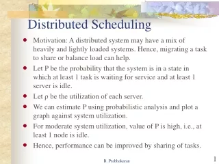
21. Dynamic Scheduling The Goal of dynamic scheduling is to load share and balance dynamically. This goal is achieved by migrating tasks from heavily loaded processors to lightly loaded processors. • Two types of task migration algorithms: • Sender-initiated • - Transfer policy (when to transfer?) • - Selection policy (which task to transfer?) • - Location policy (where to transfer?) • Potentially unstable. • Receiver-initiated CSC 8420 Advanced Operating Systems Georgia State University Yi Pan

22. Real-time Scheduling Real-time Scheduling Definitions A real-time task consists of Si, the earliest start time, Di, the deadline to finish the task and Ci, the worst-case completion time. A set of real-time tasks is called a real-time task set or a real-time system. A system of real-time tasks is called hard real-time system if all of the tasks in the system must complete execution within their respective deadlines. Even if one task misses its deadline, the whole system is considered incorrectly executed. A system of real-time tasks is called soft real-time system if the performance is judged by how many tasks missed deadline and by how much. CSC 8420 Advanced Operating Systems Georgia State University Yi Pan

23. Real-time Scheduling Real-time Scheduling Definitions A schedule for a real-time system is a CPU assignment to the tasks of the system such that a CPU is assigned to no more than one task at one time. A schedule for a real-time system is called valid if no task is assigned CPU before its earliest-start time and all tasks complete execution within their respective deadlines. A real-time system is called feasible if there is a valid schedule for the system. CSC 8420 Advanced Operating Systems Georgia State University Yi Pan

24. Real-Time Scheduling • Real-time task TASKi=(Si, Ci, Di) • Si – earliest possible start time • Ci – worst-case execution time • Di – deadline • Set of tasks V = {TASKi | I =1, …., n}

25. Aperiodic – arrive at arbitrary time • Periodic – arrival time, execution time and deadline are predictable • V = {Ji = (Ci, Ti) } • Where Ci is the execution time and Ti is the period time.

26. A schedule is a set of execution intervals • A = {(si, fi, TASKi) | i =1, …. n} • si – actual start time • fi – actual finish time • TASKi – the task executed in the time interval

27. Valid Schedule if • For every i, si < fi • For every i, fi <= si+1 • If TASKi = k, then Sk <= si and fi <= Dk (within its time interval)

28. Rate Monotonic Scheduling • Assume t is the request time for task TASKi • TASKi can meet its deadline if the time spent executing higher-priority tasks during the time interval (t,t+Di) is Di-Ci or less. • Critical instant for task TASKi occurs when task TASKi and all higher-priority tasks are scheduled simultaneously.

29. If task TASKi can meet its deadline at a critical instant, then it cal always meet its deadline. • Considering schedulability of task TASKl if we move the request time of higher-priority tasks TASKh slightly forward. • Might reduce the time spent executing TASKh in the interval (t,t+DTASKl), but not increasing .

30. Considering schedulability of task TASKl if we move the request time of higher-priority tasks TASKh slightly backward. • Might reduce the time spent executing TASKh in the interval (t,t+DTASKl), but not increasing . • Hence, at the critical instant, the amount of time spent by high-PR tasks is maximized.

31. We can now determine if a priority assignment results in a feasible schedule by simulating the execution of the tasks at the critical instant of the lowest priority task. • If the lowest-PR task can meet its deadline starting from its critical deadline, all tasks will.

32. Tasks with short periods have less time in which to complete their execution than tasks with longer deadlines. • Hence, give them higher priority. • Rate Monotonic Priority Assignment: • If Th < Tl then PRh > PRl

33. If there is a static PR assignment such that any resulting schedule is feasible, the Rate Monotonic PR Assignment policy will produce feasible schedule. • It is optimal in this sense. • How to prove? Using exchange policy for TASKi and TASKi+1.