Download
1 / 43
470 likes | 766 Views
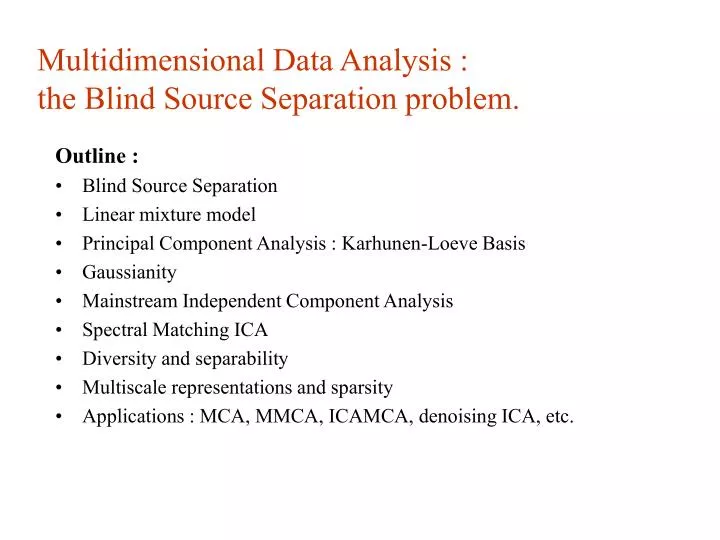
Multidimensional Data Analysis : the Blind Source Separation problem. Outline : Blind Source Separation Linear mixture model Principal Component Analysis : Karhunen-Loeve Basis Gaussianity Mainstream Independent Component Analysis Spectral Matching ICA Diversity and separability

E N D
Multidimensional Data Analysis :the Blind Source Separation problem. Outline : • Blind Source Separation • Linear mixture model • Principal Component Analysis : Karhunen-Loeve Basis • Gaussianity • Mainstream Independent Component Analysis • Spectral Matching ICA • Diversity and separability • Multiscale representations and sparsity • Applications : MCA, MMCA, ICAMCA, denoising ICA, etc.
Blind Source Separation Examples : • The cocktail party problem
Blind Source Separation Examples : • The cocktail party problem • Foregrounds in Cosmic Microwave Background imaging • Detector noise • Galactic dust • Synchrotron • Free - Free • Point Sources • Thermal SZ • …
Blind Source Separation Examples : • The cocktail party problem • Foregrounds in Cosmic Microwave Background imaging • Fetal heartbeat estimation
Blind Source Separation Examples : • The cocktail party problem • Foregrounds in Cosmic Microwave Background imaging • Fetal heartbeat estimation • Hyperspectral imaging for remote sensing
Blind Source Separation Examples : • The cocktail party problem • Foregrounds in Cosmic Microwave Background imaging • Fetal heartbeat estimation • Hyperspectral imaging for remote sensing Differentes views on a single scene obtained with different instruments. COHERENT DATA PROCESSING IS REQUIRED
A simple mixture model • linear, static and instantaneous mixture • map observed in a given frequency band sums the contributions of various components • the contributions of a component to two different detectors differ only in intensity. • additive noise • all maps are at the same resolution
23 GHz Synchrotron Free-free CMB 33 GHz 41 GHz 94 GHz A simple mixture model
23 GHz Synchrotron Free-free CMB 33 GHz 41 GHz 94 GHz A simple mixture model
Foreground removal as a source separation problem. • Processing coherent observations. • All component maps are valuable ! • How much prior knowledge? • Mixing matrix, component and noise spatial covariances known [Tegmark96, Hobson98]. • Subsets of parameters known. • Blind Source Separation assuming independent processes [Baccigalupi00, Maino92, Kuruoglu03, Delabrouille03]. • Huge amounts of high dimensional data.
Simplifying assumption • The noiseless case : X = AS • Can A and S be estimated (up to sign, scale and permutation indeterminacy) from an observed sample of X? Solution is not unique. Prior information is needed.
Karhunen-Loeve Transform a.k.a.Principal Component Analysis • Estimation of A and S assuming uncorrelated sources and orthogonal mixing matrix. • Practically : • Compute the covariance matrix of the data X • Perform an SVD : the estimated eigenvectors are the lines of A • Adaptive approximation. • Dimensionality reduction; • Used for compression and noise reduction.
Application : original image
Application : KL basis estimated from 12 by 12 patches.
Application : keeping 10 percent of basis elementscompression
Application : keeping 50 percent of basis elementscompression
Independent Component Analysis • Still in the noiseless case : X = AS • Goal is to find a matrix B such that the entries of Y = BX are independent. • Existence/Uniqueness : • Most often, such a decomposition does not exist. • Theorem [Darmois, Linnik 1950] : Let S be a random vector with independent entries of which at most when is Gaussian, and C an invertible matrix. If the entries of Y = CS are independent, then C is almost the identity. Goal will be to find a matrix B such that the entries of Y = BX are as independent as possible.
Independence or De-correlation? • Independence : • Mutual information or an approximation is used to assess statistical independence: • De-correlation measures linear independence: E( (x - E(x)) (y - E(y)) ) = 0
ICA for gaussian processes? Two linearly mixed independent Gaussian processes do not separate uniquely into two independent components. Need diversity from elsewhere. Different classes of ICA methods • Algorithms based on non-gaussianity i.e. higher order statistics. Most mainstream ICA techniques: fastICA, Jade, Infomax, etc. • Techniques based on the diversity (non proportionality) of variance (energy) profiles in a given representation such as in time, space, Fourier, wavelet : joint diagonalization of covariance matrices, SMICA, etc.
Example : Jade • First, whitening : remove linear dependencies
Example : Jade • First, whitening : removes linear dependencies, and normalizes the variance of the projected data. • Then, minimize a measure of statistical dependence ie by finding a rotation that minimizes fourth order cross-cumulants.
Example : Jade • First, whitening : removes linear dependencies, and normalizes the variance of the projected data. • Then, minimize a measure of statistical dependence ie by finding a rotation that minimizes fourth order cross-cumulants.
Application to SZ cluster map restoration Input maps
Application to SZ cluster map restoration Simulated map Output map
ICA of a mixture of independent Gaussian, stationary, colored processes (1) • Same mixture model in Fourier Space : X(l) = A S(l) • Parameters : the n*n mixing matrix A and the n • power spectra DSi(l), for l = 1 to T . • Whittle approximation to the likelihood :
ICA of a mixture of independent Gaussian, stationary, colored processes (2) • Assuming the spectra are constant over symmetric subintervals, maximizing the likelihood is the same as minimizing: • D turns out to be the Kulback Leibler divergence between two gaussian distributions. • After minimizing with respect to the source spectra, we are left with a joint diagonality criterion to be minimized wrt B = A-1. There are fast algorithms.
A Gaussian stationary ICA approach to the foreground removal problem? • CMB is modeled as a Gaussian Stationary process over the sky. • Working with covariance matrices achieves massive data reduction, and the spatial power spectra are the main parameters of interest. • Easy extension to the case of noisy mixtures. • Connection with Maximum-Likelihood guarantees some kind of optimality. • Suggests using EM algorithm. • [Snoussi2004, Cardoso2002, Delabrouille2003]
Spectral Matching ICA • Back to the case of noisy mixtures : • Fit the model spectral covariances : • to estimated spectral covariances : • by minimizing : • with respect to :
Algorithm • EM can become very slow, especially as noise parameters become small. • Speed up convergence with a few BFGS steps. • All /part of the parameters can be estimated.
Estimating component maps • Wiener filtering in each frequency band : • In case of high SNR, use pseudo inverse :
A variation on SMICA using wavelets • Motivations : • Some components, and noise are a priori not stationary. • Galactic components appear correlated. • Emission laws may not be constant over the whole sky. • Incomplete sky coverage.
A variation on SMICA using wavelets • Motivations : • Some components, and noise are a priori not stationary. • Galactic components are spatially correlated. • Emission laws may not be constant over the whole sky. • Incomplete sky coverage.
A variation on SMICA using wavelets • Motivations : • Some components, and noise are a priori not stationary. • Galactic components appear correlated. • Emission laws may not be constant over the whole sky. • Incomplete sky coverage.
A variation on SMICA using wavelets • Motivations : • Some components, and noise are a priori not stationary. • Galactic components appear correlated. • Emission laws may not be constant over the whole sky. • Incomplete sky coverage. Use wavelets to preserve space-scale information.
The à trous wavelet transform • shift invariant transform • coefficient maps are the same size as the original map • isotropic • small compact supports of wavelet and scaling functions (B3 spline) • Fast algorithms
wSMICA Model structure is not changed : Objective function : Same minimization using EM algorithm and BFGS.
Experiments Simulated Planck HFI observations at high galactic latitudes : Component maps Mixing matrix Planck HFI nominal noise levels
Experiments Simulated Planck HFI observations at high galactic latitudes :
Experiments Contribution of each component to each mixture as a function of spatial frequency :
Results Jade wSMICA initial maps
Results Errors on the estimated emission laws :
Results Rejection rates : where