Download
1 / 40
440 likes | 1.23k Views
Groundwater Remediation Lecture NOTE 10 (Multiphase Fluid Systems). Joonhong Park Yonsei CEE Department 2013. 12. 03. Saturation and Wettability. Saturation: the relative abundance of fluid in a porous medium as the volume of the i th fluid per unit void volume. S i =V i / V voids

E N D
Groundwater Remediation Lecture NOTE 10 (Multiphase Fluid Systems) Joonhong Park Yonsei CEE Department 2013. 12. 03
Saturation and Wettability • Saturation: the relative abundance of fluid in a porous medium as the volume of the i th fluid per unit void volume. Si =Vi / Vvoids • Wettability: the tendency for one fluid to be attracted to a surface in preference to another.
Interfacial Tension and Surface Tension Fluid Phase I Surface Tension < 90o Fluid Phase II Interfacial Tension Nonwetting liquid Solid Phase > 90o Wetting liquid
Interfacial Tension • When a liquid is in contact with another substance (liquid or solid), there is free interfacial energy between them, due to largely to the difference between the inward attraction of that that molecule in the interior of each phase. • Definition: the work required to separate a unit area of one substance from that of another and is expressed as a force per unit length. • Values range from zero for completely miscible liquids to 72 dynes/cm (0.072 N/m), which is the value for water at 25oC. Values for most DNAPLs range between 15 – 50 dynes/cm. • Interfacial tension, σ = ρhrg/2 • Here ρ = the liquid density; h = capillary rise; • r= the radius of the tube; g=the acceleration due to gravity
Capillary Forces • Definition: The pressure discontinuity across any curved interface separating two immiscible fluids. • Pc = Pnw –Pw = 2σ/r • A measure of the tendency of a porous medium to imbibe the wetting phase or to repel the nonwetting phase.
Imbibition and Drainage • Hysteresis • Effect of hydraulic conductivity (Figure 19.3)
Relative Permeability qi = (ki/μi) ( Pi – ρi g h) qi = (kkri/μi) ( Pi – ρi g h) kri = (ki/k): Demond and Roberts, 1987 Here k: intrinsic permeability kri : relative permeability ki : the effective permeability of the medium to the i th fluid. Function of (intrinsic permeability; pore size distribution; viscosity ratio; interfacial tension; wettability)
Relative Permeability 1.0 0.0 Snw 1.0 krn kri krw Drainage Imbibition 0.5 0.0 Sw 1.0 + krw < 1 (1) krn and krw = 0 (no flow) at residual saturations (2) krn
Residual Saturation (Sr) and krw = 0.0 (no flow) when Srn and Srw krn Typically Srn < Srw Insular Saturation For nonwetting fluid Pendular Saturation for wetting fluid
Relative Permeability 1.0 0.0 Snw 1.0 krn kri krw Drainage Imbibition 0.5 0.0 Sw 1.0 (3) krn > krw REASON: Nonwetting occupies larger pores while wetting does smaller ones. REASON: Nonwetting occupies a different pore network during imbibition than during drainage. (4) hysteresis for krn
Relative Permeability 1.0 0.0 Snw 1.0 krn kri krw Drainage Imbibition 0.5 0.0 Sw 1.0 (5) Residual Srn(oil):Saturated(0.1-0.5) > Vadose(0.1-0.2) (6) The permeability shape = f (intrinsic k, pore size dist., viscosity ratio, interfacial tension, wettability)
Volumetric retention capacity, Rc A measure of the ‘potential’ of the unsaturated zone to trap NAPL. Rc = 1000 Sr * n Rc: the volumetric retention capacity (liters of NAPL per m3) Sr: the residual saturation of the NAPL n: porosity Rc increases with decreasing moisture content, effective porosity, and intrinsic permeability.
Solubility and Effective Solubility In general, organic pollutants are mixed together in field. The Theoretical upper limit dissolved phase concentration of a constituent in equilibrium with ground water = Xi * Si Xi: mole fraction of a component i in a DNAPL mix. Si: pure phase solubility of component i.
Light NAPL (non-aqueous phase liquid) contamination Tank LNAPL residual Vapor from LNAPL Capillary fringe LNAPL Free Phase Water table Dissolved LNAPL (plume) Groundwater Flow
Conceptual Models for LNAPLs • True thickness vs. Apparent thickness • Horizontal preferential flows due to differences in K values • Horizontal preferential flows through capillary fringe. • Effect of GW table fluctuations (a significant NAPL can be trapped by a rising water table.
Dense NAPL contamination Vapor from NAPL NAPL residual Capillary fringe Water table Dissolved NAPL (plume) Clay Layer Groundwater Flow Direction LNAPL Free Phase Groundwater Flow DNALP to upstream Fractured rock
Relative ease of cleaning-up of contaminated aquifers as a function of contaminant chemistry and hydrogeology (1=easiest; 4 = the most difficult) Contaminant chemistry Strongly sorbed, dissolved (degrades/volatilizes) Strongly sorbed, dissolved Separate Phase LNAPL Separate Phase DNAPL Mobile, Dissolved (degrades/ Volatilizes) Mobile, Dissolved Hydrogeology Homogeneous, single layer 1 1-2 2 2-3 2-3 3 Homogeneous, multiple layer 1 1-2 2 2-3 2-3 3 Heterogeneous, single layer 2 2 3 3 3 4 Heterogeneous, multiple layer 2 2 3 3 3 4 Fractured 3 3 3 3 4 4
NAPLs Quantitative Methods • Volume of aquifer containing residual • The depth L of the residual given above • Depth of residual in a fracture • Height of a DNAPL pool that can be supported by low permeability lens • Height of DNAPL pool that can be supported by a fractured capillary barrier • Thickness of DNAPL on the capillary fringe to cause DNAPL to enter the saturated zone • Critical DNAPL thickness for entry into a fracture at the top of the saturated zone • The time required to dissolve a DNAPL pool in the saturated zone.
Contaminant distribution among multiple phases in environment FOR distribution of a solute (species A) between multi-phases @ equilibrium (used for heterogeneous rxn) Gas & Water : Henry constant, KH PA = KH * CA, (Pi= [ni/ V]*R*T) here, P=partial pressure, C=molar conc. Water & Organic phase: Partition Coeff., Kp CA in organic = Kp * CA in water Solid & Water: Q = KF * Cwn in water (or = KD Cw) Ksp=[A]a[B]b Aqueous Solubility, Cs: Max. concentration of a solute in water Vapor Pressure, PO : Max. concentration of a solute in air
Vapor pressure (I) Def.) The vapor pressure of a pure liquid species is the equilibrium partial pressure of the gas molecules of that species above a flat surface of the pure liquid. Water vapor V PH2O nH2O PH2OV = nH2ORT nH2O/V = PH2O/RT Water PoH2O @equilibrium
Dissolution of Species in Water Partitioning between Gas Phase and Water: Henry’s Law
Dissolution of Species in Water Partitioning between Gas Phase and Water: Henry’s Law Example: Saturation concentration of oxygen in water Compute the equilibrium mass concentration of oxygen (O2) in units of mg/L for water exposed to the atmosphere at sea level at a temperature of 15oC. (At 15oC, KH,O2 = 654 atm/M, partial pressure O2 in air = 0.209 ) Solution: Since P = 1atm at sea level, PO2 =0.209 * 1atm PO2 = KH, O2 * CO2, w CO2, w = PO2/KH,O2 = 0.209 (atm)/654 (atm/M) = 0.000320 M Mass Concentration = Molarity * Oxygen MW = 0.000320 (M) * 32(g/mol) * 1000(mg/g) = 10.2 mg/L
Dissolution of Species in Water Partitioning between Gas Phase and Water: Henry’s Law Example: Partitioning of toluene in a closed system A 2L glass jar is half filled with water and half filled with air at a temperature of 293K. After 92 mg (=10-3mol) of liquid toluene is added, the jar is sealed. (1) What is the equilibrium concentration of toluene in the water? And (2) what is the equilibrium partial pressure of toluene in the gas phase? (KH for toluene, KH,tol, @ 20oC = 6.7 atm/M) Solution: Henry’s law Ptol = KH,tol * Ctol,w => Ctol,w = Ptol/KH,tol Ideal gas law Ptol * Vg = nRT => Ctol,g = (n/Vg) = Ptot/RT Material balance: Ctol, w * Vw + Ctol, g * Vg = Total amount of toluene (Ptot /KH,tol)* Vw + Ptol* Vg/(RT) = 0.0010 mol Ptot = 0.0052 atm => Ctot,g = 0.0052/(0.0821*293) =0.00022 M Ctot,w = 0.00078 M
Henry’s law Real behavior Raoult’s law Ideal Solution Law Fugacity, fi,j: a tendency of a species i to escape from phase j. Raoult’s law (the 1st ideal solution law): governs the behavior of pure or nearly pure solid or liquid substances with respect to pure vapor phase Henry’s law (the 2nd idea solution law): governs the behavior of dilute solutions with respect with the vapor pressure of species i. Fugacity, fi,j 0.0 0.5 1.0 Mole fraction, Xi in j phase
Dissolution of Species in Water Solubility of Nonaqueous-Phase Liquids (NAPLs) NAPL: liquids that do not mix with water (e.g. spills of petroleum products or organic solvents) Aqueous solubility @ a temperature, Cs. Xylene phase Xylene Distribution of Xylene Raoult’s law Cs Xylene Water phase
Dissolution of Species in Water When a small amount of xylene was spilled, no free phase exists. Xylene-air, Water-air Fugacity of Xylene from air Henry’s law Fugacity of H2O from water Raoult’s law Air phase Xylene-water, Air-water Water phase When a large amount of xylene was spilled, a free phase exists. Xylene-air = Po, Water-air Air phase Air-xylene, Water-xylene Distribution of Xylene Raoult’s law (Non-Aqueous Phase Liquids [NAPLs]) Xylene phase Xylene-water = Cs, Air-water Water phase
Dissolution of Species in Water Solubility of Nonaqueous-Phase Liquids (NAPLs) • Example: Dissolution of a NAPL • 1 L of liquid toluene (density =87g/cm3) is spilled into 1 m3 of water. Assuming no loss of toluene or water from the system, what is the steady-state concentration of toluene dissolved in the water? • Repeat (a) assuming that the water volume is 10 m3. • [Hint: Cs of toluene = 530 mg/L] • Solution: • [1000 cm3 of toluene * 0.87 g/cm3]/[1000 L of water] = 870 mg/L > Cs • The toluene concentration in water cannot be higher than Cs. Therefore, toluene concentration in water should be Cs. • Residual NAPL remains. • (b) 870 g/10,000L = 87 mg/L < Cs • No NAPL is left.
SORPTION: Absorption versus Adsorption Intra-phase solute distribution Bulk Phase Bulk Phase v v Homogeneous surface, constant surface energy ADsorbing Phase ABsorbing Phase Interface Solute Accumulation Heterogeneous surface, distributed surface energies
ABsorption: Partitioning Coefficient KP: partitioning coefficient i: compound i phase 1 phase 2 Octanol-water partition coefficient (often used as a measure of “hydrophobicity”) Empirical constants
Adsorption • Definition: the accumulation of dissolved substances at interfaces of and between phases. • Solvent-motivated adsorption: surface tension and interfacial tension. • Sorbent-motivated adsorption: • Chemical adsorption • Electrostatic adsorption • Physical adsorption
Models for describing sorption equilibria Sorption Isotherms: plots of resulting data relating the variation of solid-phase concentration to the variation of solution-phase concentration at a fixed temperature. Favorable Qe Eq. Conc. In Solid Linear Unfavorable Ce Eq. Conc. In Solution M: the initial mass of a species Ce:Eq. Concentration of a species in solution Vw: volume of solution (liquid portion only) m:the amount of sorbent
Adsorption model (I) Linear Model Distribution coefficient. Qe Equil. Conc. in Solid. Mass fraction of organic carbon. Empirical coefficients. Ce Equil. Conc. in Water.
Adsorption Model (II) For solid-water system Qe Qeo Max. sorption capacity 0.5*Qeo Langmuir model (half saturation constant) KL Ce
Adsorption Model (III): Freundlich Model • Sorption of solute in water-soil system is not well described by theoretical models such as linear and Langmuir. • Heinrich Freundlich and other investigators suggested that data for solutions are frequently best described by a general exponential concentration-dependent relationship of the form 0< n <1 Qe n = 1 n >1
Multiple phase distribution of a species Example: 10-3 mol of toluene was spilled in a 2L sealed jar, half filled with water and half filled with air. The equilibrium partitioning was described by Henry’s law, so that the aqueous phase contained 0.00078 M and 0.00022 M. To this system, 200 mg of activated carbon was added. Toluene partitioning between the sorbed and aqueous phases was described by the Freundlich isotherm Qe =100 Cw0.45 where Ce is the aqueous concentration in mg/L and Qe is the sorbed mass concentration in mg-toluene per g-activated carbon. What is the new equilibrium concentration of toluene in the water? How much of activated carbon is needed to reduce Cw into 0.000008M? Total amt of toluene = Qe*(amt of a.c.) + Cw*Vw +Cg*Vg = KF * Cwn * (amt of a.c.) + Cw*Vw + KHO*Cw*Vg Air phase 1L Water phase 1L 200 mg of activated carbon (a.c.)
Fate of Organics in Unsaturated Zone • Volatilization • Gas Transport by Diffusion (see Eq.19.13-19) • Equilibrium Calculations of Mass Distribution • M-aqueous = n-wr * C-water • M-soil = soil (dried) bulk density * C-soil • M-NAPL=n-nr * NAPL density • M-gas=n-gas * C-gas • here C-gas = n/V = P/RT (mol/L) : convert to mg/L
Fate of Organics in Saturated Zone Total mass = amount in solution (water) + amount sorbed + amount in NAPL Total mass = C-water *(n - n-nr) + C-soil*soil bulk density + n-nr * NAPL density
Air Permeability Testing Typical set up for the test (Figure 20.26) Figure 19.36 => P’ =A ln t + B During the air permeability tests, at least one pore volume of vapor should be removed. Vp = ngasπ R2 H R: the radius of the contaminated zone H: the thickness of the contaminated zone
Recognizing DNAPL Sites • Site use and history • Groundwater zone sampling for free product (NAPL-water interface probes, inspection of the pumped fluid or samples collected by transparent bottom-loading bailers or depth-discrete samplers [EPA, 1992]) • Anomalously high dissolved concentration (greater than 1% of effective solubility [EPA, 1992]) • Soil sampling (> 1% soil mass) • Cw in saturated soil = M * ρb / (Kd*ρb + nw) (Cw > effective solubility of the NAPL) • Systematic Screening Procedure (EPA method; Figure 19.27-29)