Download

1 / 47
470 likes | 606 Views
Delay-Optimal Precoder Adaptation for Multi-stream MIMO Systems in Wireless Fading Channels. Vincent Lau Dept of ECE Hong Kong University of Science and Technology. Outline. Introduction System Model Markov Decision Problem Formulation and Challenges Multi-Level Water-Filling Solution

E N D
Delay-Optimal Precoder Adaptation for Multi-stream MIMO Systems in Wireless Fading Channels Vincent Lau Dept of ECE Hong Kong University of Science and Technology
Outline • Introduction • System Model • Markov Decision Problem Formulation and Challenges • Multi-Level Water-Filling Solution • Numerical Results • Conclusion
Outline • Introduction • Why Delay is Important • Using MIMO to Boost PHY Layer Performance • The Scenario of Multi-stream MIMO Link • Related Works & Remaining Challenges • System Model • Markov Decision Problem Formulation and Challenges • Multi-Level Water-Filling Solution • Numerical Results • Conclusion
Introduction • Why delay performance is important? • “WHAT??!! He is stuck in the air?? !$*&(#@&@#!!” • “You must be kidding me! Buffering at such an important moment!!??” You Tube Conclusion I: Real-life applications are delay-sensitive!!
Introduction • We may have multiple delay-sensitive wireless applications running at the same time! Play multi-player game Keep track of a game Conclusion II: Different applications have heterogeneousdelay-requirement Keep talking to some friends
Introduction • MIMO is well-known to boost the PHY Performance Wireless Fading Channel SISO MIMO Encoder MIMO Decoder • Spatial Multiplexing Gain • Diversity Gain Wireless Fading Channel MIMO
Introduction • Using MIMO to Boost PHY Layer Performance S/P STBC/SM MIMO Detector Wireless Fading Channel Q) How is this related to Delay? Can’t we just use conventional technique in MIMO to boost the PHY performance? If the PHY is improved, the delay of the application will be improved as well. NO CSIT Wireless Fading Channel S/P MIMO Precoder & Power Control MIMO Detector Perfect CSIT
Introduction • Multi-stream MIMO Link Delay REQ 1 MIMO Precoder & Power Adaptor Fring Packets Wireless Fading Channel G-MAP Packets Delay REQ 2 YouTube Packets Delay REQ L Queueing State Information (QSI) Channel State Information (CSI)
Related Works • Traditional MIMO precoder design for PHY • [Sampath’01], [Scaglione’99],[Palomar’03], etc. • Linear MIMO precoder design framework to minimize the weighted sum of mean square errors (MSE) assuming knowledge of perfect CSIT. • In general, optimal precoder may not always diagonalize the channel Remark: Only adapt based on CSIT only, ignoring queue states and optimize PHY layer only metric • [Love’05], [Lau’04], [Rey’05], [Palomar’04], etc. • MIMO precoder design with limited feedback. • MIMO adaptation design with outdated CSIT. [Kittipiyakul’04] : naive water-filling, which is optimal in information theoretical sense, is not always a good strategy w.r.t. the delay performance. Conclusion: Very important to make use of both (channel state info) CSI and (queue state info) QSI for delay sensitive applications
Introduction • Challenges to incorporate QSI and CSI in adaptation • Challenge 1: Requires both the Information theory (modeling of the PHY dynamics) & the Queueingtheory (modeling of the delay/buffer dynamics) • Challenge 2: Brute-force approach cannot lead to any viable solution Information Theory Queueing Theory Leonard Kleinrock Claude Shannon When Shannon meets Kleinrock…
Related Works • Various approaches dealing with delay problems • Approach I : Stability Region and Lynapnov Drift [Berry’02], [Neely’07], etc. • Discuss stability region of point-to-point SISO and multiuser SISO. • Also considered asymptotically delay-optimal control policy based on “Lynapnov Drift” • The authors obtained interesting tradeoff results as well as insight into the structure of the optimal control policy at large delay regime. Remark: This approach allows simple control policy with design insights but the control will be good only for asymptotically large delay regime. v -v S<1/v S>1/v Buffer State s To regulate the buffer state towards 1/v
Related Works • Various approaches dealing with delay problems Approach II [Yeh’01], [Yeh’03] - Symmetric and homogeneous users in multi-access fading channels - Using stochastic majorization theory, the authors showed that the longest queue highest possible rate (LQHPR) policy is delay-optimal A Capacity region B higher rate for user 1 Longer queue for user 1
Related Works • Various approaches dealing with delay problems Approach III : [Wu’03], [Hui’07], [Tang’07], etc. To convert the delay constraint into average rate constraint using tail probability at large delay regime and solve the optimization problem using information theoretical formulation based on the rate constraint. Remark: While this approach allows potentially simple solution, the control policy will be a function of CSIT only and such control will be good only for large delay regime. Note: In general, the delay-optimal power and precoder adaptation should be a function of both the CSI and the QSI.
Related Works • Various approaches dealing with delay problems Approach IV : [Bertsekas’87] The problem of finding the optimal control policy (to minimize delay) is cast into a Markov Decision Problem (MDP) or a stochastic control problem. • Remark: • Unfortunately, it is well-known that there is no easy solution to MDP in general. • Brute-force value iteration and policy iteration are very complex and time-consuming. • In addition, it is usually very complex to evaluate the optimal solution even numerically.
Related Works • Technical Challenges to be Solved Challenge 1: Low complexity optimal control policy for delay sensitive resource allocation problem in general delay regime. • Remark 1: • Most of the existing works considered large delay asymptotic solutions. • However, practical operating region for delay sensitive traffics are usually on the low delay regime and hence the asymptotic simplifications cannot be applied. • Therefore, it is important to obtain low complexity control policy for general delay regime. • Brute force optimization is challenging because (a) the problem is not convex; (b) huge dimension of variables involved; (c) Not able to express the average delay in terms of the control variables.
Related Works • Remaining Challenges to be Solved Challenge 2: Coupling among multiple delay-sensitive heterogeneous data streams. • Remark 2: • Most of the above works considered single stream wireless link only. • While [Yeh’01], [Yeh’03] considered multi-access systems, the framework applies to situations with homogeneous users only and cannot be extended to situations with heterogeneous users. • When we have heterogeneous data streams, the problem will be difficult as the optimal policy will generally be coupled with the joint queue state of all the heterogeneous streams. • And the general solution involves solving multi-dimensional MDP with exponential order of complexity w.r.t. the number of streams.
Related Works • Remaining Challenges to be Solved Challenge 3: Delay-sensitive MIMO precoder design with outdated CSIT. • Remark 3: • In practice, CSIT is not perfect. • There will be spatial interference between the MIMO channels. • The MIMO precoder design for delay-sensitive applications will be difficult because the resulting SINR of the spatial channels are coupled together with different delay requirements among the spatial streams.
Outline • Introduction • System Model • MIMO Physical Layer Model • Queue Model & System States • Objective & Control Policy • Markov Decision Problem Formulation • Low Complexity Solution • Numerical Results • Conclusion
System Model • Multi-Stream MIMO Physical Layer Model Linear Precoder Linear Equalizer Imperfect CSI
System Model • Imperfect CSIT • Imperfect CSIT in FDD System: • CSIT is obtained by explicit feedback. • CSIT is imperfect due to the limited feedback bits constraint • Imperfect CSTI in TDD System: • CSIT is obtained by implicit feedback using the channel reciprocal property between the forward and reverse link. • CSIT is imperfect due to estimation noise and the duplexing delay. -- reverse link pilot SNR • Perfect CSIT : • No CSIT :
System Model • MIMO Physical Layer Model Equivalent channel (P, H, W) for the L data stream: Conditional average SINR of the i-th data stream: Conditional symbol error probability for QAM constellation: Wiener filter Simultaneously maximize MIMO PHY Layer Precoder P Data rate (bits per symbol) of the i-th data stream:
System Model • Queue Dynamics & System States G-MAP Packets MAC State QSI YouTube Packets MIMO Precoding Control Action Cross Layer MIMO Precoding Controller MAC Layer CSI MIMO Precoder time PHY Layer PHY State Packet Arrivals PHY Frames • Channel is quasi-static in a slot • i.i.d between slots
System Model the service rate of the L streams are coupled together because of the precoderP • Objective & Control Policy M/M/1 Queue System parameters: Poisson arrival with rate: Average packet length: (exponentially dist.) • Challenges: • Huge dimension of variables involved • Exponential State Space • No closed form expression for average delay (in terms of precoder) Based on P Definitions: Average delay of the i-th stream: Average power constraint: Positive weighting factors (Pareto Optimal Tradeoff) Lagrange multiplier for the average power constraint Optimization problem: Delay Optimal Policy
Outline • Introduction • System Model • Markov Decision Problem Formulation and Challenges • Embedded Markov Chain & MDP Formulation • Bellman Condition & Optimal Precoding Structure • Optimal Power Allocation Policy • Summary of the Optimal Solution • Multi-level Water-filling Solution • Numerical Results • Conclusion
Markov Decision Problem Formulation • Overview of MDP (Stochastic Dynamic Programming) Key Idea: Divide-and-Conquer To break a large problem (optimization over the policy space) into smaller problem (optimization over a control action at a stage).
Markov Decision Problem Formulation • Specification of an Infinite Horizon Markov Decision Problem • Decisions are made at points of time – decision epochs • System state and Control Action Space: • At the t-th decision epoch, the system occupies a state • The controller observes the current state and applies an action • Per-stage Reward & Transition Probability • By choosing action the system receives a reward • The system state at the next epoch is determined by a transition probability kernel • Stationary Control Policy: • The set of actions for all system state realizations • The Optimization Problem: • Average Reward • Optimal Policy
Markov Decision Problem Formulation • Solution of an Markov Decision Problem Key Criterion: Bellman’s Equation Under some technical conditions, the optimal value of the problem is given by the solution of the Bellman’s Equation.
Markov Decision Problem Formulation • Infinite Horizon MDP Structure of our Precoder Problem • Our Decision Epoch: Time slots • Our System State at the m-th slot: • Our Control action at the m-th slot: Precoder • Our Per stage “reward”: • Our Average “reward” (average delay): decision epoch decision epoch System state action reward Control policy L-stream MIMO system time
Markov Decision Problem Formulation • Our Transition Probability Kernel: • For a given control policy ,the sequence of joint queue state observed at each time slot is an L-dim controlled Markov Chain. • Due to the different time scales on slot duration and packet arrival / departure process, at the -th decision epoch, only one of the following events can happen: • Event 1: • Packet arrival from the i-th data source • Poisson arrival assumption for all streams • Event 2: • Packet arrival from the i-th data source • Poisson arrival assumption for all streams • Event 3: • Nothing happens
Markov Decision Problem Formulation • Our Transition Probability Kernel: State transition diagram for L-dimension Markov chain {Qm} with N states each dimension. L=2 for illustration. The induced Markov Chain is “aperiodic” and “irreducible”.
Delay-Optimal MIMO Precoding Solution • Two Major Challenges • 1) continuous state space (CSI): • Most of the results in MDP theory applies to countable state space only. Extension to continuous state space is not trivial. • 2) Exponentially large Q state (QSI): • The total number of states in the joint-queue-state (QSI) = N^L • Exponentially large complexity and memory requirement = O(exp[L])!!
Challenge (I) – Reduced State MDP • Solution 1) Reduced State MDP • One challenge of the MDP problem is the continuous state space (CSI). • Most of MDP solutions require finite state space. • Observe that given a control policy , the induced markov chain {Q(m)} only depends on the control via the “conditional average service rate” We could have an equivalent “reduced state MDP” (evolves based on the finite state space Q)
Challenge (I) – Reduced State MDP • Bellman Condition & Optimal Precoding Structure • Optimal solution is obtained by the Bellman’s equation
Challenge (I) – Reduced State MDP • Optimal Precoding Structure Delay Optimal Precoder still has a “MIMO channel Diagonaling Structure”
Challenge (I) – Reduced State MDP • Remaining Problem is to solve for power allocation across the L streams • Optimal power allocation policy • “Multi-level” water-filling type solution • “Water-filling” based on the CSI • “Water level” depends on the QSI (indirectly via
Challenge (I) – Reduced State MDP • How to obtain the “water-level” ? • Solving the Bellman Equation (23) ~ • Exponential complexity and memory requirement w.r.t L (# of data streams) Not a scalable solution
Challenge (II) – Decomposition of MDP • The coupling of the L-dimension MDP is due to the “dynamic sorting of eigenvalues” according to • Associate the largest eigenchannel to the stream with the largest . • To reduce the complexity of the solution, we restrict to “static sorting” of eigenvalues. • Associate the largest eigenchannel to the stream with the largest and so on… Lemma 3: (Additive Property): Based on “static sorting” policy, the solution to the Bellman’s equation has the form
Challenge (II) – Decomposition of MDP • As a result, the Bellman’s equation can be decomposed into L 1-D Bellman’s equation: • Exploiting the Birth-Death Queue Dynamics, the 1-D Bellman’s equation can be solved recursively (easily):
Low Complexity Solution – Offline Solution • Offline Solution ~ Complexity O(L) Outputs of the Offline Procedure
Low Complexity Solution – Online Procedure Instantaneous CSI & QSI of L-streams Memory storing results of Offline Solution (O[L]) MIMO Precoder & Power Allocation
Outline • Introduction • System Model • Markov Decision Problem Formulation • Low Complexity Solution • Numerical Results • Optimal Solution v.s. Low Complexity Solution • Different Antenna Configurations • Impact of the CSIT Error Variance • Conclusion
Numerical Results • How much performance loss if using the low complexity solution? • Condition: • No. of data streams : 2 • Buffer length : 4 • Arrival rate : 0.02 p/ch use • Frame Duration: 5 ms • Target SER : 0.01 • Weighting factors : 1 / 10 • Average packet size: 200 bits • Remark: • Support heterogeneous delay application • “static sorting” achieves near optimal performance.
Numerical Results • How is the low complexity performance under different antenna configuration? • Condition: • No. of data streams : 2 • Buffer length : 4 • Arrival rate : 0.02 p/ch use • Frame duration: 5 ms • Target SER : 0.01 • Weighting factors : 1 / 10 • Average packet size: 200 bits • Remark: • Delay comparison w. r. t. MIMO configuration
Numerical Results • How is the low complexity performance compared with different baselines? • Condition: • No. of data streams : 2 • Buffer length : 4 • Arrival rate : 0.02 p/ch use • Frame Duration: 5 ms • Target SER : 0.01 • Weighting factors : 1 / 10 • Average packet size: 200 bits gain • Remark: • Better performance than the two baselines: • Round-Robin • Traditional MIMO precoding(CSIT only) • Robust to CSIT errors
Outline • Introduction • System Model • Markov Decision Problem Formulation • Low Complexity Solution • Numerical Results • Conclusion
Conclusion Conclusion 1: Delay-Optimal MIMO Precoder – a function of both CSI and QSI with channel diagonalizing structure. Conclusion 2: Delay-Optimal Power Allocation – multilevel water-filling: Water-filling across CSI, water level determined by QSI. Conclusion 3: Proposed a “reduced state MDP” to deal with the continuous state space challenge Conclusion 4: Proposed a “static-sorting scheme” to decompose MDP low complexity algorithm O(L) to obtain “water-levels”.
Thank you!Questions are Welcomed! Vincent Lau – eeknlau@ust.hk