Download
1 / 26
260 likes | 311 Views
What is Statistics?. Statistics, in short, is the study of data . Croxton & Cowden have given a very simple and

E N D
What is Statistics? Statistics, in short, is the study of data. Croxton & Cowden have given a very simple and concise definition of statistics ,In their view, “ Statistics may be defined as a science of collection, presentation, analysis and interpretation of numerical data.
Characteristics of Statistics: • Statistics should deal with aggregate of individuals. • Statistics should be expressed as numerical figures. • Statistics should have the property of being varied by multiplicity of causes. • Statistics collected should be of reasonable standards of accuracy. • Statistics should be obtained for pre- determined purpose. • Statistics collected should allow comparison with other data.
Scope of Statistics: Statistics in Business: • Applications of statistics permeate almost every area of activity in business & industry such as marketing, production, financial analysis, distribution analysis, market research, research & development, manpower planning & accounting.
Limitation of Statistics • Statistics does not deals with isolated measurement. • Statistics deals with only the quantitative characteristic. • Statistical results are true only on an average. • Statistics can be misused.
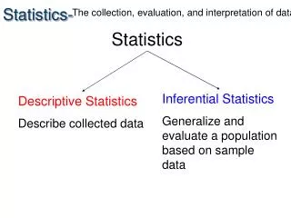
Basic types of Statistics: There are two basic types of statistics such as • Descriptive Statistics • Inferential Statistics • Descriptive statistics: • Descriptive statistics refers to methods of organizing, summarizing, and presenting data in an informative way. • Example 1: • A Gallup poll found that 49% of the people in a survey knew the name of the first book of the Bible. The statistic 49 describes the number out of every 100 persons who knew the answer. • Inferential statistics: • Inferential statistics is a decision, estimate, guess, or generalization about a population, based on a sample.
Types of data • There are two types of data. Such as • Primary data • Secondary data • Primary data: • They refer to those which are collected a fresh and for the first time, and thus happen to be original in character. • Secondary data: They refer to those which have already been collected by someone else and which have already been passed through the statistical process.
Description of Variable • Qualitative variable or Attribute: • This refers to the attribute or characteristic that is nonnumeric. • Example: Gender, religious affiliation and eye color. • Quantitative variable: • This refers to a variable that can be reported numerically. • Example: Balance in your, income, wages, and number of children in a family. • Quantitative variables can be classified as: • Discrete • Continuous • Discrete variables: • Discrete variables are generally counts and can take on only discrete values. Normally they are represented by natural numbers .
Example • Example: 1: • The number of bedrooms in a house. (1, 2, 3... etc...). • If the number of children in a family is the variable of interest, it is obvious that it cannot assume fractional values and hence it is a discrete variable. The important point is that the possible values of the variable are separated from one another.
Example • Continuous variables: • A variable is said to be continuous if it can theoretically assume any value within given range or ranges. • Example: • The time it takes to fly from Dhaka to New York. Other examples include height of a person, price of a commodity and time.
Example • The following data relate to the number of refrigerators sold a 22 working days by a leading house. • 23, 30, 20, 26, 30, 30, 20, 23, 40, 40, 26, 20, 23,40, 28, 26, 23, 30, 40, 28, 28, 30. • From the above data, prepare a frequency distribution table • Frequency distribution of the Number of Refrigerators Sold • No. of Refrigerators Tally Bars Frequency (No. of days) • 20 /// 3 • 23 //// 4 • 26 /// 3 • 28 /// 3 • 30 ///// 5 • 40 //// 4 • Total 22
Class limits: • The class limits are the lowest and the highest values that can be included in the class. • Example: • Take the class 20-40. The lowest value of this class is 20 and the highest 40. The two boundaries of a class are known as the lower limit and upper limit of the class. The lower limit of a class is the value below which there can be no value in that class.
Class–intervals: • The span of a class that is the difference between the upper limit and the lower limit is known as class –interval. • Example: • In the class 20-40, the class interval is 20 (i.e., 40 minus 20). • Class frequency: • The number of observations corresponding to the particular class is known as the frequency of that class or the class frequency. For example, the frequency of the class 5000-6000 is 50 ( as mentioned in slide ch.3-23) which implies that there are 50 employees having income between Tk.5000 and Tk. 6000.
Class mid-point: • It is the value lying half-way between the lower and upper class limits of a class–interval. Mid-point of a class is ascertained as follows: • Mid-point of a class = (Upper limit+ Lower limit)/2 • Exclusive method • Inclusive method
What are methods of classifying the data according to class intervals? • Exclusive method • Inclusive method • Exclusive method: • Under the ‘exclusive’ method of classification, the upper limit of one class is the lower limit of the next class. • Income (Tk) No. Employees • 5000-6000 50 • 6000-7000 100 • 7000-8000 200 • 8000-9000 150 • 9000-10000 40 • 10000-11000 10 • Total 550
Inclusive Method: • Inclusive Method: • Under the ‘inclusive’ method of classification, the upper limit of one class is included in that class itself. • Income (Tk) No. Employees • 5000-5999 50 • 6000-6999 100 • 7000-7999 200 • 8000-8999 150 • 9000-9999 40 • 10000-10999 10 • Example • 20,22,35,42,37,42,48,53,49,65,39,48,67,18,16,23,37,35,49,63, 65, 55, 45,58,57,69,25,29,58,65. • Classify the above data takinga suitable class- interval. • Solution: • Let us determine the suitable class-interval with the help of the following formulas:
Solution: Since values like, 3, 7, 9, etc. should be avoided and therefore, we will take 10 as the class-interval and the first class as 15-25.
Profits (Tk. Lac) Tally Bar No of Companies • 15-25 //// 5 • 25-35 // 2 • 35-45 /////// 7 • 45-55 ///// 6 • 55-65 ///// 5 • 65-75 ///// 5
Histogram: • A graph in which the classes are marked on the horizontal axis and the class frequencies on the vertical axis. The class frequencies are represented by the heights of the bars and the bars are drawn adjoining to each other. • Class Size Frequency • 0-10 5 • 10-20 11 • 20-30 19 • 30-40 21 • 40-50 17 • 50-60 10 • 60-70 8 • 70-80 6 • 90-100 1
Ogive Curve: • A cumulative frequency distribution (ogive) is used to determine how many or what proportion of the data values are below or above a certain value. • From the following frequency distribution, prepare the ‘less than’ and ‘more than’ cumulative frequency distribution (ogive curve). Hours each student spent Number of students per day studies 0-10 8 10-20 12 20-30 30 30-40 25 40-50 18 50-60 17
The frequency distribution is arranged for ogive by less than method, as mentioned below: • Cumulative frequency dist. Of students by hours spend on studies
The frequency distribution is arranged for ogive by more than method, as mentioned below: • Cumulative frequency distribution of students by hours spent by students
Hours each student spent Number of students More than CF Hour spent • per day studies • 0-10 8 110 Less than 0 • 10-20 12 102 10 • 20-30 30 90 20 • 30-40 25 60 30 • 40-50 18 35 40 • 50-60 17 17 50