Download
1 / 34
340 likes | 345 Views
This lecture covers queuing theory, including the head-cylinder software queue, disk latency, and Little's Law. It also introduces the concept of multiprocessing in computer architecture.

E N D
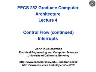
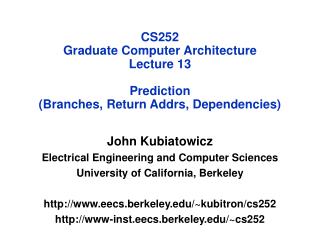
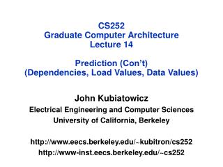
CS252Graduate Computer ArchitectureLecture 19Queuing Theory (Con’t)Intro to Multiprocessing John Kubiatowicz Electrical Engineering and Computer Sciences University of California, Berkeley http://www.eecs.berkeley.edu/~kubitron/cs252
Head Cylinder Software Queue (Device Driver) Hardware Controller Media Time (Seek+Rot+Xfer) Request Result Track Recall: Magnetic Disk Characteristic Sector • Cylinder: all the tracks under the head at a given point on all surface • Read/write data is a three-stage process: • Seek time: position the head/arm over the proper track (into proper cylinder) • Rotational latency: wait for the desired sectorto rotate under the read/write head • Transfer time: transfer a block of bits (sector)under the read-write head • Disk Latency = Queueing Time + Controller time + Seek Time + Rotation Time + Xfer Time • Highest Bandwidth: • transfer large group of blocks sequentially from one track Platter cs252-S09, Lecture 19
Controller Disk Queue Departures Arrivals Queuing System Recall: Introduction to Queuing Theory • What about queuing time?? • Let’s apply some queuing theory • Queuing Theory applies to long term, steady state behavior Arrival rate = Departure rate • Little’s Law: Mean # tasks in system = arrival rate x mean response time • Observed by many, Little was first to prove • Simple interpretation: you should see the same number of tasks in queue when entering as when leaving. • Applies to any system in equilibrium, as long as nothing in black box is creating or destroying tasks • Typical queuing theory doesn’t deal with transient behavior, only steady-state behavior cs252-S09, Lecture 19
Queue Server Arrival Rate Service Rate μ=1/Tser A Little Queuing Theory: Mean Wait Time • Parameters that describe our system: • : mean number of arriving customers/second • Tser: mean time to service a customer (“m1”) • C: squared coefficient of variance = 2/m12 • μ: service rate = 1/Tser • u: server utilization (0u1): u = /μ = Tser • Parameters we wish to compute: • Tq: Time spent in queue • Lq: Length of queue = Tq (by Little’s law) • Basic Approach: • Customers before us must finish; mean time = Lq Tser • If something at server, takes m1(z) to complete on avg • Chance server busy = u mean time is u m1(z) • Computation of wait time in queue (Tq): • Tq = Lq Tser + u m1(z) cs252-S09, Lecture 19
Total time for n services … T1 T2 T3 Tn Random Arrival Point Mean Residual Wait Time: m1(z) • Imagine n samples • There are n P(Tx) samples of size Tx • Total space of samples of size Tx: • Total time for n services: • Chance arrive in service of length Tx: • Avg remaining time if land in Tx: ½Tx • Finally: Average Residual Time m1(z): cs252-S09, Lecture 19
Little’s Law Defn of utilization (u) A Little Queuing Theory: M/G/1 and M/M/1 • Computation of wait time in queue (Tq): Tq = Lq Tser + u m1(z) Tq = Tq Tser + u m1(z) Tq = u Tq + u m1(z) Tq (1 – u) = m1(z) u Tq = m1(z) u/(1-u) Tq = Tser ½(1+C) u/(1 – u) • Notice that as u1, Tq ! • Assumptions so far: • System in equilibrium; No limit to the queue: works First-In-First-Out • Time between two successive arrivals in line are random and memoryless: (M for C=1 exponentially random) • Server can start on next customer immediately after prior finishes • General service distribution (no restrictions), 1 server: • Called M/G/1 queue: Tq = Tser x ½(1+C) x u/(1 – u)) • Memoryless service distribution (C = 1): • Called M/M/1 queue: Tq = Tser x u/(1 – u) cs252-S09, Lecture 19
A Little Queuing Theory: An Example • Example Usage Statistics: • User requests 10 x 8KB disk I/Os per second • Requests & service exponentially distributed (C=1.0) • Avg. service = 20 ms (From controller+seek+rot+trans) • Questions: • How utilized is the disk? • Ans: server utilization, u = Tser • What is the average time spent in the queue? • Ans: Tq • What is the number of requests in the queue? • Ans: Lq • What is the avg response time for disk request? • Ans: Tsys = Tq + Tser • Computation: (avg # arriving customers/s) = 10/s Tser(avg time to service customer) = 20 ms (0.02s) u (server utilization) = x Tser= 10/s x .02s = 0.2 Tq(avg time/customer in queue) = Tser x u/(1 – u) = 20 x 0.2/(1-0.2) = 20 x 0.25 = 5 ms (0 .005s) Lq (avg length of queue) = x Tq=10/s x .005s = 0.05 Tsys(avg time/customer in system) =Tq + Tser= 25 ms cs252-S09, Lecture 19
Use Arrays of Small Disks? • Katz and Patterson asked in 1987: • Can smaller disks be used to close gap in performance between disks and CPUs? Conventional: 4 disk designs 3.5” 5.25” 10” 14” High End Low End Disk Array: 1 disk design 3.5” cs252-S09, Lecture 19
Array Reliability • Reliability of N disks = Reliability of 1 Disk ÷ N 50,000 Hours ÷ 70 disks = 700 hours Disk system MTTF: Drops from 6 years to 1 month! • Arrays (without redundancy) too unreliable to be useful! Hot spares support reconstruction in parallel with access: very high media availability can be achieved cs252-S09, Lecture 19
Redundant Arrays of DisksRAID 1: Disk Mirroring/Shadowing recovery group • Each disk is fully duplicated onto its "shadow" Very high availability can be achieved • Bandwidth sacrifice on write: Logical write = two physical writes • Reads may be optimized • Most expensive solution: 100% capacity overhead Targeted for high I/O rate , high availability environments cs252-S09, Lecture 19
Redundant Arrays of Disks RAID 5+: High I/O Rate Parity Increasing Logical Disk Addresses D0 D1 D2 D3 P A logical write becomes four physical I/Os Independent writes possible because of interleaved parity Reed-Solomon Codes ("Q") for protection during reconstruction D4 D5 D6 P D7 D8 D9 P D10 D11 D12 P D13 D14 D15 Stripe P D16 D17 D18 D19 Targeted for mixed applications Stripe Unit D20 D21 D22 D23 P . . . . . . . . . . . . . . . Disk Columns cs252-S09, Lecture 19
Problems of Disk Arrays: Small Writes RAID-5: Small Write Algorithm 1 Logical Write = 2 Physical Reads + 2 Physical Writes D0 D1 D2 D0' D3 P old data new data old parity (1. Read) (2. Read) XOR + + XOR (3. Write) (4. Write) D0' D1 D2 D3 P' cs252-S09, Lecture 19
System Availability: Orthogonal RAIDs Array Controller String Controller . . . String Controller . . . String Controller . . . String Controller . . . String Controller . . . String Controller . . . Data Recovery Group: unit of data redundancy Redundant Support Components: fans, power supplies, controller, cables End to End Data Integrity: internal parity protected data paths cs252-S09, Lecture 19
Administrivia • Still grading Exams! • Sorry – my TA was preparing for Quals • Will get them done in next week (promise!) • Projects: • Should be getting fully up to speed on project • Set up meeting with me this week cs252-S09, Lecture 19
What is Parallel Architecture? • A parallel computer is a collection of processing elements that cooperate to solve large problems • Most important new element: It is all about communication! • What does the programmer (or OS or Compiler writer) think about? • Models of computation: • PRAM? BSP? Sequential Consistency? • Resource Allocation: • how powerful are the elements? • how much memory? • What mechanisms must be in hardware vs software • What does a single processor look like? • High performance general purpose processor • SIMD processor/Vector Processor • Data access, Communication and Synchronization • how do the elements cooperate and communicate? • how are data transmitted between processors? • what are the abstractions and primitives for cooperation? cs252-S09, Lecture 19
Flynn’s Classification (1966) Broad classification of parallel computing systems • SISD: Single Instruction, Single Data • conventional uniprocessor • SIMD: Single Instruction, Multiple Data • one instruction stream, multiple data paths • distributed memory SIMD (MPP, DAP, CM-1&2, Maspar) • shared memory SIMD (STARAN, vector computers) • MIMD: Multiple Instruction, Multiple Data • message passing machines (Transputers, nCube, CM-5) • non-cache-coherent shared memory machines (BBN Butterfly, T3D) • cache-coherent shared memory machines (Sequent, Sun Starfire, SGI Origin) • MISD: Multiple Instruction, Single Data • Not a practical configuration cs252-S09, Lecture 19
P P P P Bus Memory P/M P/M P/M P/M P/M P/M P/M P/M P/M P/M P/M P/M Host P/M P/M P/M P/M Network Examples of MIMD Machines • Symmetric Multiprocessor • Multiple processors in box with shared memory communication • Current MultiCore chips like this • Every processor runs copy of OS • Non-uniform shared-memory with separate I/O through host • Multiple processors • Each with local memory • general scalable network • Extremely light “OS” on node provides simple services • Scheduling/synchronization • Network-accessible host for I/O • Cluster • Many independent machine connected with general network • Communication through messages cs252-S09, Lecture 19
Categories of Thread Execution Simultaneous Multithreading Multiprocessing Superscalar Fine-Grained Coarse-Grained Time (processor cycle) Thread 1 Thread 3 Thread 5 Thread 2 Thread 4 Idle slot cs252-S09, Lecture 19
Parallel Programming Models • Programming model is made up of the languages and libraries that create an abstract view of the machine • Control • How is parallelismcreated? • What orderings exist between operations? • How do different threads of control synchronize? • Data • What data is privatevs.shared? • How is logically shared data accessed or communicated? • Synchronization • What operations can be used to coordinate parallelism • What are the atomic (indivisible) operations? • Cost • How do we account for the costof each of the above? cs252-S09, Lecture 19
A = array of all data fA = f(A) s = sum(fA) A: f fA: sum Simple Programming Example • Consider applying a functionf to the elements of an array A and then computing its sum: • Questions: • Where does A live? All in single memory? Partitioned? • What work will be done by each processors? • They need to coordinate to get a single result, how? s: cs252-S09, Lecture 19
Shared memory s s = ... y = ..s ... i: 5 i: 8 i: 2 Private memory P1 Pn P0 Programming Model 1: Shared Memory • Program is a collection of threads of control. • Can be created dynamically, mid-execution, in some languages • Each thread has a set of private variables, e.g., local stack variables • Also a set of shared variables, e.g., static variables, shared common blocks, or global heap. • Threads communicate implicitly by writing and reading shared variables. • Threads coordinate by synchronizing on shared variables cs252-S09, Lecture 19
Simple Programming Example: SM • Shared memory strategy: • small number p << n=size(A) processors • attached to single memory • Parallel Decomposition: • Each evaluation and each partial sum is a task. • Assign n/p numbers to each of p procs • Each computes independent “private” results and partial sum. • Collect the p partial sums and compute a global sum. Two Classes of Data: • Logically Shared • The original n numbers, the global sum. • Logically Private • The individual function evaluations. • What about the individual partial sums? cs252-S09, Lecture 19
Shared Memory “Code” for sum static int s = 0; Thread 1 for i = 0, n/2-1 s = s + f(A[i]) Thread 2 for i = n/2, n-1 s = s + f(A[i]) • Problem is a race condition on variable s in the program • A race condition or data race occurs when: • two processors (or two threads) access the same variable, and at least one does a write. • The accesses are concurrent (not synchronized) so they could happen simultaneously cs252-S09, Lecture 19
A Closer Look A 3 5 f = square static int s = 0; Thread 1 …. compute f([A[i]) and put in reg0 reg1 = s reg1 = reg1 + reg0 s = reg1 … Thread 2 … compute f([A[i]) and put in reg0 reg1 = s reg1 = reg1 + reg0 s = reg1 … 9 25 0 0 9 25 9 25 • Assume A = [3,5], f is the square function, and s=0 initially • For this program to work, s should be 34 at the end • but it may be 34,9, or 25 • The atomic operations are reads and writes • Never see ½ of one number, but += operation is not atomic • All computations happen in (private) registers cs252-S09, Lecture 19
static lock lk; lock(lk); lock(lk); unlock(lk); unlock(lk); Improved Code for Sum static int s = 0; Thread 1 local_s1= 0 for i = 0, n/2-1 local_s1 = local_s1 + f(A[i]) s = s + local_s1 Thread 2 local_s2 = 0 for i = n/2, n-1 local_s2= local_s2 + f(A[i]) s = s +local_s2 • Since addition is associative, it’s OK to rearrange order • Most computation is on private variables • Sharing frequency is also reduced, which might improve speed • But there is still a race condition on the update of shared s • The race condition can be fixed by adding locks (only one thread can hold a lock at a time; others wait for it) cs252-S09, Lecture 19
What about Synchronization? • All shared-memory programs need synchronization • Barrier – global (/coordinated) synchronization • simple use of barriers -- all threads hit the same one work_on_my_subgrid(); barrier; read_neighboring_values(); barrier; • Mutexes – mutual exclusion locks • threads are mostly independent and must access common data lock *l = alloc_and_init(); /* shared */ lock(l); access data unlock(l); • Need atomic operations bigger than loads/stores • Actually – Dijkstra’s algorithm can get by with only loads/stores, but this is quite complex (and doesn’t work under all circumstances) • Example: atomic swap, test-and-test-and-set • Another Option: Transactional memory • Hardware equivalent of optimistic concurrency • Some think that this is the answer to all parallel programming cs252-S09, Lecture 19
Private memory receive Pn,s s: 11 s: 14 s: 12 y = ..s ... i: 3 i: 2 i: 1 send P1,s P1 Pn P0 Network Programming Model 2: Message Passing • Program consists of a collection of named processes. • Usually fixed at program startup time • Thread of control plus local address space -- NO shared data. • Logically shared data is partitioned over local processes. • Processes communicate by explicit send/receive pairs • Coordination is implicit in every communication event. • MPI (Message Passing Interface) is the most commonly used SW cs252-S09, Lecture 19
Second possible solution Processor 2 xloadl = A[2] receive xremote, proc1 send xlocal, proc1 s = xlocal + xremote Processor 1 xlocal = A[1] send xlocal, proc2 receive xremote, proc2 s = xlocal + xremote Compute A[1]+A[2] on each processor • First possible solution – what could go wrong? Processor 1 xlocal = A[1] send xlocal, proc2 receive xremote, proc2 s = xlocal + xremote Processor 2 xlocal = A[2] send xlocal, proc1 receive xremote, proc1 s = xlocal + xremote • If send/receive acts like the telephone system? The post office? • What if there are more than 2 processors? cs252-S09, Lecture 19
MPI – the de facto standard • MPI has become the de facto standard for parallel computing using message passing • Example: for(i=1;i<numprocs;i++) { sprintf(buff, "Hello %d! ", i); MPI_Send(buff, BUFSIZE, MPI_CHAR, i, TAG, MPI_COMM_WORLD); } for(i=1;i<numprocs;i++) { MPI_Recv(buff, BUFSIZE, MPI_CHAR, i, TAG, MPI_COMM_WORLD, &stat); printf("%d: %s\n", myid, buff); } • Pros and Cons of standards • MPI created finally a standard for applications development in the HPC community portability • The MPI standard is a least common denominator building on mid-80s technology, so may discourage innovation cs252-S09, Lecture 19
Which is better? SM or MP? • Which is better, Shared Memory or Message Passing? • Depends on the program! • Both are “communication Turing complete” • i.e. can build Shared Memory with Message Passing and vice-versa • Advantages of Shared Memory: • Implicit communication (loads/stores) • Low overhead when cached • Disadvantages of Shared Memory: • Complex to build in way that scales well • Requires synchronization operations • Hard to control data placement within caching system • Advantages of Message Passing • Explicit Communication (sending/receiving of messages) • Easier to control data placement (no automatic caching) • Disadvantages of Message Passing • Message passing overhead can be quite high • More complex to program • Introduces question of reception technique (interrupts/polling) cs252-S09, Lecture 19
Basic Definitions • Network interface • Processor (or programmer’s) interface to the network • Mechanism for injecting packets/removing packets • Links • Bundle of wires or fibers that carries a signal • May have separate wires for clocking • Switches • connects fixed number of input channels to fixed number of output channels • Can have a serious impact on latency, saturation, deadlock cs252-S09, Lecture 19
...ABC123 => ...QR67 => Receiver Transmitter Links and Channels • transmitter converts stream of digital symbols into signal that is driven down the link • receiver converts it back • tran/rcv share physical protocol • trans + link + rcv form Channel for digital info flow between switches • link-level protocol segments stream of symbols into larger units: packets or messages (framing) • node-level protocol embeds commands for dest communication assist within packet cs252-S09, Lecture 19
Data Req Ack Transmitter Asserts Data t0 t1 t2 t3 t4 t5 Clock Synchronization? • Receiver must be synchronized to transmitter • To know when to latch data • Fully Synchronous • Same clock and phase: Isochronous • Same clock, different phase: Mesochronous • High-speed serial links work this way • Use of encoding (8B/10B) to ensure sufficient high-frequency component for clock recovery • Fully Asynchronous • No clock: Request/Ack signals • Different clock: Need some sort of clock recovery? cs252-S09, Lecture 19
Conclusion • Disk Time = queue + controller + seek + rotate + transfer • Queuing Latency: • M/M/1 and M/G/1 queues: simplest to analyze • Assume memoryless input stream of requests • As utilization approaches 100%, latency • M/M/1: Tq = Tser x u/(1 – u) • M/G/1: Tq = Tser x ½(1+C) x u/(1 – u) • Multiprocessing • Multiple processors connect together • It is all about communication! • Programming Models: • Shared Memory • Message Passing cs252-S09, Lecture 19