Download
1 / 35
350 likes | 444 Views
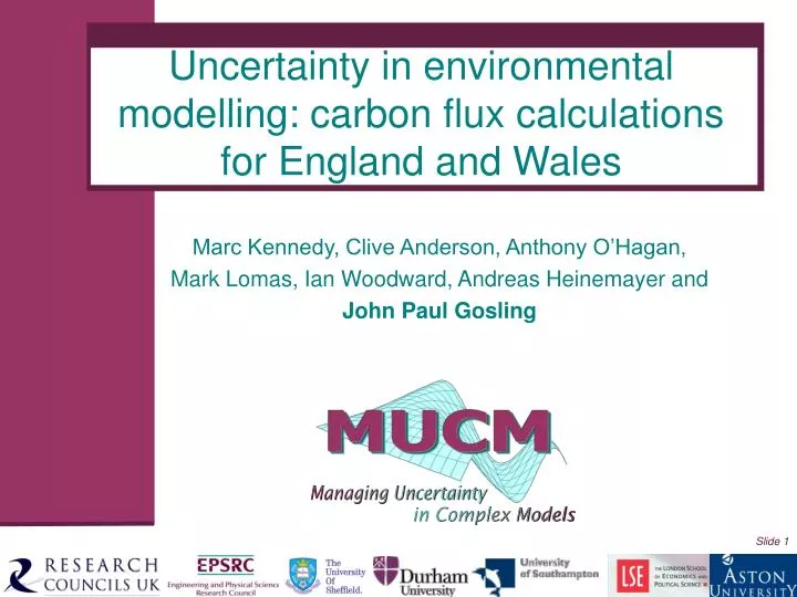
Uncertainty in environmental modelling: carbon flux calculations for England and Wales. Marc Kennedy, Clive Anderson, Anthony O’Hagan, Mark Lomas, Ian Woodward, Andreas Heinemayer and John Paul Gosling. This talk. Carbon flux in England and Wales Sources of uncertainty

E N D
Uncertainty in environmental modelling: carbon flux calculations for England and Wales Marc Kennedy, Clive Anderson, Anthony O’Hagan, Mark Lomas, Ian Woodward, Andreas Heinemayer and John Paul Gosling
This talk • Carbon flux in England and Wales • Sources of uncertainty • Dealing with uncertainty • Results (so far) • Further research
Carbon Flux • Carbon flux (CF) is the exchange of carbon between the land (vegetation and soils) and the atmosphere. • Gross primary production (GPP) is a measure of photosynthetic fixation by vegetation of CO2. • Net biome productivity (NBP) is the net uptake of carbon by the land (i.e. vegetation and soil).
NBP in pictures Vegetation extracts carbon from the atmosphere. This is given as GPP.
NBP in pictures Vegetation and soil respire; this adds carbon back into the atmosphere.
NBP in pictures Disturbances can negatively affect this process.
NBP in pictures Disturbances can negatively affect this process.
NBP in pictures NBP = GPP – plant respiration – soil respiration – disturbances
Previous attempts to quantify CF • Some studies have focused on particular plant functional types, e.g. woodland, and particular areas of the UK. • Others have tried to quantify it in extremely small areas with respect to England and Wales. • Dynamic vegetation models (DVMs) have been employed to calculate CF as have techniques of inversion on the atmospheric CO2 levels.
What do we want to know about? • What was the NBP for England and Wales in the year 2000? • Not just a guess – even if it is a well educated guess using sophisticated models and super computers. • A mean for NBP AND a measure of our uncertainty.
Our results • Mean NBP of 7.55 MtC • A standard deviation of 0.56 MtC for NBP • Basic idea: Use a simulator of the physical processes (or computer code) to inform us about the actual NBP value.
SDGVM • The simulator we used for this study was the Sheffield Dynamic Global Vegetation Model (SDGVM). • The simulator can be represented as a function: η(X) = Y where X is a vector of inputs and Y is the model output.
Where does the uncertainty come from? • We consider two main sources of uncertainty: we do not know η(X) for every possible X therefore we are uncertain about η(.), we do not know the correct values of X for the simulator.
Uncertainty in computer code outputs – a GP model • Our prior uncertainty about the simulator is given by a Gaussian process: • These beliefs are updated using training data from the simulator.
Uncertainty in computer code outputs – what does SDGVM give us? • England and Wales is divided into squares with 1/6th of a degree length. • We consider NBP for the situation where each square is completely covered by • Grassland • Crops • Deciduous broadleaf trees • Evergreen needle leaf trees • Essentially, we have a function that represents SDGVM for each PFT at each site.
Uncertainty in computer code outputs – aggregation of outputs • We are interested in the total NBP for England and Wales in the year 2000, which is given by: where is the area of site i and is the proportion of PFT t at site i. • Uncertainty about the simulator and its inputs must be propagated through this sum.
Uncertainty in computer code outputs – computational restrictions • Using an emulator allows us to run just the simulator a fraction of the times in comparison to a Monte Carlo method. • However, to emulate well, we need approximately 900 simulator runs per site. 707 * 900 simulator runs = 636300 simulator runs (This would take about 440 days as one simulator run takes approximately 1 min)
Uncertainty in moving from 33 to 707 sites • Sample sites: varied climatic conditions cover the whole region adequately wide range of land cover types different inter-site distances
Uncertainty in moving from 33 to 707 sites - kriging • We cannot simply interpolate across the whole of England and Wales using some standard regression technique as we wish to capture all our uncertainty. • Kriging has been about for many years in geostatistics, and it is analogous to the Gaussian process techniques we use to model the simulator.
Uncertainty in moving from 33 to 707 sites - kriging • We want to report mean NBP and its variance for each site. • We get a posterior mean value for the non-sample sites. • We also get a measure of our about NBP uncertainty at each non-sample site. • In order to perform kriging, we must specify a spatial correlation structure. This can be done in a fully probabilistic manner; however, we actually just estimated the covariograms using the sample sites.
Uncertainty in computer code inputs • Our uncertainty in the simulator inputs drives some of our uncertainty about the simulator output. Y = η(X) • Effort must be made to accurately elicit our beliefs about X.
Uncertainty in computer code inputs – parameter types • There are three main parameter types that SDGVM uses: • Plant inputs • There are 4 plant functional types (PFTs): grassland, crop, deciduous broad leaf and evergreen needle leaf. • Soil inputs • These are location specific, i.e. what are the average soil characteristics at that particular site. • Climate data
Uncertainty in computer code inputs – sensitivity analysis • We use sensitivity analysis techniques that exploit properties of the Gaussian process model to establish which simulator inputs actually have an impact on NBP. • We then spent time eliciting expert beliefs about those important inputs. • This exercise led to many adjustments to the simulator as we explored parts of the input space the simulator builders had never considered.
Uncertainty in computer code inputs – soil parameters • Soil texture and bulk density parameters must be specified for each simulator run. • The important soil parameters were found to be sand percentage, clay percentage and bulk density. • We use the same soil parameters for each PFT. • For each of the sample sites, soil data were available at 1 km2 resolution, giving a number of observations of the relevant parameters for each site.
Uncertainty in computer code inputs – plant parameters • Different numbers of plant-type inputs were found to be important for each PFT. • There was not the same kind of data available as there was for the soil parameters. • The plant parameters were assumed to be the same across England and Wales. • We elicited distributions for these from an expert.
Uncertainty in computer code inputs – climate forcing data • For SDGVM, the climate inputs are interpolated climate records or climate models. • In this study, monthly temperature, precipitation, air humidity and cloudiness for the year 2000 from the CRU/UEA dataset were used. • Monthly data are downscaled to a daily time-step with a weather generator. • The climate data is assumed to be known with no uncertainty………………………………..
Uncertainty in computer code inputs – sensitivity analysis Expected output for each input after integrating out uncertainty from other inputs. This is for DcBl at site 3 (Middlesbrough area)
NBP results in colour Mean (gC/m2) Standard deviation (gC/m2)
Our results vs. previous results • Previous attempts have been limited to specific areas within what we have covered in this analysis. • We have expressed a measure of uncertainty about NBP and not just given a point estimate. • But our results are far from being perfect….
Uncertainty in the land cover map • We used:
Uncertainty in the climate forcing data • We used observed climate data to drive SDGVM. • Observed data taken as being known. • We had to move from monthly to daily data on precipitation using a simple stochastic model –a first order Markov chain for the sequence of wet and dry days and then the amount drawn from a gamma distribution.
Uncertainty in SDGVM’s connection with reality • SDGVM is a perfect representation of reality.
Uncertainty in SDGVM’s connection with reality • SDGVM is a perfect representation of reality. • I think not! • We have to think about model discrepancy. • This is extremely difficult especially when we have no data on the same scale on which we are modelling.
References • Kennedy, M.C., Anderson, C.W., O'Hagan, A., Lomas, M.R., Woodward, F.I., Heinemeyer, A. and Gosling, J.P. (2006). Quantifying uncertainty in the biospheric carbon flux for England and Wales. To appear in J. R. Statist. Soc. Ser. A. • Gosling, J.P. and O’Hagan, A. (2006). Understanding the uncertainty in the biospheric carbon flux for England and Wales. Research report 567/06, Department of Probability and Statistics, University of Sheffield, Sheffield, UK. Both of these and software to help you get started with UA and SA for computer models can be found on: www.tonyohagan.co.uk