Download
1 / 27
270 likes | 389 Views
Learn the intricacies of high-order surface construction, including smoothness, flexibility, local parameterization, spline-based vs. manifold-based approaches, and detailed steps for efficient surface construction methods. Understand the importance of smoothness, flexibility, and local parameterization in achieving visually appealing surfaces with accurate computation results.

E N D
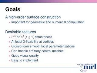
Goals • A high-order surface construction • Important for geometric and numerical computation • Desirable features • or smoothness • At least 3-flexibility at vertices • Closed-form smooth local parameterizations • Can handle arbitrary control meshes • Good visual quality • Easy to implement
Smoothness • smoothness • A standard goal in CAGD important for high-accuracy computation • Computing surface properties • : needed for normal • : needed for curvatures, reflection lines; • : needed for curvature variation;
Flexibility • Ability to represent local geometry • Property of basis function, instead of the surface • Two-Flexibility: any desired curvature at any point 1-flexible 2-flexible Todo: replace with shaded picture
Local Parameterization • Explicit smooth local parameterization • For any point, there is an explicit formula defining the surface in a neighborhood of this point • Simplifies many tasks • Defining functions on surfaces • Integration over surfaces • Surface-surface intersections • Computing geodesics
Spline-based Approach • Construct surface patch for each face • Find smooth local parameterization for every point • Difficult to guarantee smoothness for points on patch boundaries
Manifold-based Approach • Construct overlapping charts covering the mesh • Build local geometry approximating the mesh on each chart • Find blending function for each chart • Get the surface by blending local geometry … …
Basic steps • Construction has two parameters: smoothness k and n > k, defining how closely the surface follows the control mesh • We consider the case k = 2 (C2 surfaces), and n = 3 • The number of charts grows with n, so smaller is better for most applications • Steps • subdivide using Catmull-Clark 3 times • define 1 quad chart for each regular vertex not adjacent to irregular, 2 quad charts for some adjacent, K quad charts for vertices of valence K • define 1 basis function per chart • assign a 1 control point per vertex
Step 1: Subdivide • Subdivide 3 times (use Catmull-Clark) • charts will (more or less) correspond to 2-neighborhoods of vertices in the refined mesh • subdivide enough so that if charts overlap they can contain only one irregular vertex
Step 2: Define charts • If 2-neighborhood has no irregular vertices • simply map part of the mesh to a square
Step 2: Define charts • Regular vertices close to irregular (within 2 ring) • make a curved star mapping 4-nbhd of irregular vertex to the plane; irregular vertex splits into K. • sweep the outer curve of the curved 2-nbhd to get a chart
Step 2: Define charts • Regular vertices diagonal from irregular and irregular • for these vertices, the outer boundary has multiple segments; use multiple charts
Step 3: basis functions • One control point assigned per vertex • several charts may share a control point • similar to splines, weighted blend of control points • Basis functions are tensor product splines of degree k+1, remapped to the charts Quad charts make the definition easy
Step 4: transition maps • Transition maps are • affine for charts containing irregular vertices (these charts always share the same star) • affine for regular to regular chart • polynomial for regular to irregular
Summary of properties • smoothness: Ck • flexibility: unknown at irregular • charts shape: all quads • charts are associated with vertices, multiple charts for some vertices • number of charts: large;approx. 4^(subdiv steps)* # of vertices for C2 , 3 subdiv. steps, i.e. 64* # of vertices • flexibility: unknown • embedding functions: constants (1 control point/chart) • blending functions: tensor-product B-splines remapped • transition functions: linear or polynomial of degree k+1 • reduce to splines of degree k+1 for regular control meshes
Previous Work • High-order spline patches • S-patches [Loop and DeRose 1989] • DMS splines [Seidel 1994] • Freeform splines [Prautzsch 1997] • TURBS [Reif 1998] • C2 flexible subdivision surfaces • G2 subdivision [Prautzsch and Umlauf 1996] • Manifold-based approach • [Grimm and Hughes 1995] • [Navau and Garcia 2000] • [Grimm 2002]
Charts and Transition Maps • Building local geometry for one-ring neighborhood is easy • How to blend them together smoothly ? • The transition map must be smooth ? Smooth Smooth Smooth Smooth
Charts and Transition Maps • Charts • One for each vertex • Map only depends on valence • Transition maps • Conformal, thus • Easy to compute • Alternatives smooth smooth smooth transition map
Local Geometry Maps • Needs to be smooth and 3-flexible at center vertex • Use monomials as basis for local geometry • High order splines can also be used • Needs to provide good visual quality • Make it close to an existing surface with good quality • Use Catmull-Clark subdivision surface
Catmull-Clark subdivision Fitting Dyadic points Local Geometry Maps • Constraints: • 3d positions • Positions in chart • Basis • Monomials in chart • Unknowns • Monomial coefficients • Least square fitting Pseudo-inverse can be pre-computed
Blending Functions • Need to be a partition of unity • Need to be smooth in each chart tensorproduct rotate and copy map
Evaluation Procedure • Find correspondent positions in each chart • Evaluate local geometry by local chart position • Compute blending function in each chart • Blend local geometry to get surface position
Local Parameterization Local parameterization around extraordinary vertex Our surface Catmull-Clark Magnitude of derivatives 1st order 2nd order 3rd order
High-order smoothness Curvature behavior Reflection lines Catmull-Clark Our surface
Summary of Features • charts: star-shaped, depend on vertex valence • one chart per vertex • embedding functions: polynomials or splines • blending functions: compositions of conformal and polynomial • transition functions: conformal • C1 or Ck smooth for a prescribed k • At least 3-flexible at vertices • Explicit local parameterizations exist for any point