Download
1 / 25
250 likes | 364 Views
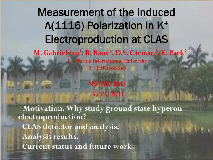
Measurement of the Induced Λ (1116) Polarization in K + Electroproduction at CLAS. M. Gabrielyan 1 , B. Raue 1 , D.S. Carman 2 , K. Park 2 Florida International University Jefferson Lab NSTAR 2011 5/19/2011. Motivation. Why study ground state hyperon electroproduction ?

E N D
Measurement of the Induced Λ(1116)Polarization in K+Electroproductionat CLAS • M. Gabrielyan1, B. Raue1, D.S. Carman2, K. Park2 • Florida International University • Jefferson Lab • NSTAR 2011 • 5/19/2011 • Motivation. Why study ground state hyperonelectroproduction? • CLAS detector and analysis. • Analysis results. • Current status and future work.
Motivation • This study is part of a larger program that has a goal of measuring as many observables as possible for KYelectroproduction. • Understand which N*’s couple to KY final states. • These data are needed in a coupled-channel analysis to identify previously unobserved N* resonances. • Get a better understanding of the strange-quark production process by mapping out the kinematic dependencies for these observables. • The results will tell us which (if any) of the currently available models best describe the data.
CEBAF Large Acceptance Spectrometer • Toroidal magnetic field in region 2 • 3 regions of drift chambers located spherically around target provide charged particle tracking for angle and momentum reconstruction • Cherenkov detectors provide e/p separation • Electromagnetic calorimeters give total energy measurement for electrons and neutrals and also e/p separation • Time of flight scintillators for particle ID
Kinematics and E1F Dataset • Beam energy = 5.5 GeV • Unpolarized Target • Torus current = 2250 A • 5B triggers, 213000 Λ’s Q2 vs W Q2 vs cos(θKCM) • 0.8 < Q2 < 3.5 GeV2 • 1.6 < W < 2.8 GeV • -1.0 < cos(θKCM) < 1.0
Particle Identification • Electrons: • Coincidence between CC and EC in the same sector. • Negatively charged track in DC that matches in time with TOF. • Momentum correctionsapplied to correct for DC misalignments and inaccuracies in the magnetic field map. • Hadrons:Timedifference (Δt) between the measured time • and the computed time for a given hadron species (p+, K+, p). MinimumΔt identifies the hadron.
Hadron Identification MinimumΔt identifies the hadron. After Λ and missing mass cuts p K+ Minimum Δt vs p
Hadron Identification MinimumΔt identifies the hadron. After Λ and missing mass cuts p given K mass p K+ Minimum Δt vs p p given K mass
Λ Identification • Reconstructed missing mass for e+pe’K+(Y) • For recoil polarization observables e+pe’K+p(p-) include p- missing-mass cut Σ(1192) Λ(1116) MM2(π-) vs MM(eK+) MM2(π-) Background in the hyperon missing mass spectrum is dominated by p’s misidentified as K+. MM(eK+)
Cross Section for Electroproduction Polarized beam & recoil Λ, unpolarized target. Where: Transferred polarization Induced polarization
Parity non-conservation in weak decay allows to extract recoil polarization from p angular distribution in Λ rest frame. where: α=0.642 ± 0.013 (PDG) ΛPolarization Extraction Here NFand NBare the acceptance corrected yields. After Φ integration onlyPN component survives for induced polarization (PL, PT = 0). Carman et al., PRC 79 065205 (2009)
Acceptance Corrections FSGen: Phase space generator with modified t-slope : t-slope = 0.3 GeV-2 Acceptance corrections are applied to background subtracted yields. 0.8<Cos(θKCM)< 1.0 MC T N DATA L W Acceptance factors vs W ΘK vs φK CM
Background Subtraction • The fit function form is motivated by theΛ and Σ Monte Carlo templates that are matched to data. • fΛ= G Λ + L ΛL+ L ΛR • f Σ= G Σ + L ΣL+ L ΣR • fBKG= A*(bkg_temp) • fTOTAL= fΛ+ fΣ+ fBKG • G Λ = Gaussian, • L ΛL = Left Lorentzian, • L ΛR = Right Lorentzian, • A = Amplitude. G Λ + L ΛL G Λ + L ΛR The background templates are generated from data by intentionally misidentifying pions as kaons.
Background Subtraction 1.05 < MM(eK+) < 1.15 GeV Λ0 N: W =2.0125 T: W=1.7375 ∑0 Cos(θKCM)=0.9 Cos(θKCM)=0.9 Bkg. Total FWD χ2 =1.063 FWD χ2 =1.003 N: W =2.0125 T: W=2.575 Cos(θKCM)=0.9 Cos(θKCM)=0.9 FWD χ2 =1.075 BKWD MM(eK+) MM(eK+)
Systematics Check: PLvsW -1.0<Cos(θKCM)<-0.5 Preliminary Results SUM over Q2, Φ 0.4<Cos(θKCM)<0.6 -0.5<Cos(θKCM)<0.0 0.6<Cos(θKCM)<0.8 0.0<Cos(θKCM)<0.2 0.8<Cos(θKCM)< 1.0 0.2<Cos(θKCM)<0.4 W W
Induced Polarization PN vs W -1.0<Cos(θKCM)<-0.5 Preliminary Results SUM over Q2, Φ <Systematics> ≤ 0.06 0.4<Cos(θKCM)<0.6 -0.5<Cos(θKCM)<0.0 0.6<Cos(θKCM)<0.8 0.0<Cos(θKCM)<0.2 0.8<Cos(θKCM)< 1.0 0.2<Cos(θKCM)<0.4 W W
RPR Model • Non-resonant background contributions treated as exchanges of kaonic Regge trajectories in the t-channel: K(494) and K*(892) dominant trajectories. Both have a rotating Regge phase. This approach reduces the number of parameters. • Included established s-channel nucleon resonances: S11(1650), P11(1710), P13(1720), P13(1900) • Included missing resonance: D13(1900). • Model was fit to forward angle (cos θKCM > 0) photoproduction data (CLAS, LEPS, GRAAL) to constrain the parameters. Corthals et al., Phys. Lett. B 656 (2007)
Induced Polarization PN vs W -1.0<Cos(θKCM)<-0.5 Preliminary Results SUM over Q2, Φ 0.4<Cos(θKCM)<0.6 -0.5<Cos(θKCM)<0.0 0.6<Cos(θKCM)<0.8 0.0<Cos(θKCM)<0.2 0.8<Cos(θKCM)< 1.0 0.2<Cos(θKCM)<0.4 W W
Induced Polarization PN vs W -1.0<Cos(θKCM)<-0.5 Preliminary Results SUM over Q2, Φ 0.4<Cos(θKCM)<0.6 -0.5<Cos(θKCM)<0.0 0.6<Cos(θKCM)<0.8 0.0<Cos(θKCM)<0.2 0.8<Cos(θKCM)< 1.0 0.2<Cos(θKCM)<0.4 W W
Induced Polarization vs W (photoproduction) Red:McCracken, CLAS 2010 Blue: McNabb, CLAS 2004 Green: Glander, SAPHIR 2004 Black: Lleres, GRAAL 2007 Dashed lines indicate the physical limits of polarization. W (GeV) M.E. McCracken et al., Phys. Rev. C 81, 025201 (2010).
Induced Polarization vs W (photoproduction) Red:McCracken, CLAS 2010 Blue: McNabb, CLAS 2004 Green: Glander, SAPHIR 2004 Black: Lleres, GRAAL 2007 Dashed lines indicate the physical limits of polarization. -0.5<Cos(θKCM)< 0.0 0.8<Cos(θKCM)< 1.0 W (GeV) M.E. McCracken et al., Phys. Rev. C 81, 025201 (2010).
SUMMARY • Background subtraction and acceptance corrections are complete. • RPR theoretical model calculations are in good agreement with experimental data at very forward kaon angles but they fail to reproduce the data at all other kaon angle bins. • RPR gives a reasonable description of photoproduction data (cos θKCM > 0). • Experimental data are similar for both electro- and photoproduction at forward kaon angles, but are very different for backward kaon angles. NEXT… • Complete the systematic error analysis. • Comparison to different theoretical models. • Funded in part by: The U.S. Dept. of Energy, FIU Graduate School
Systematics Check: PT vs W -1.0<Cos(θKCM)<-0.5 Preliminary Results SUM over Q2, Φ 0.4<Cos(θKCM)<0.6 -0.5<Cos(θKCM)<0.0 0.6<Cos(θKCM)<0.8 0.0<Cos(θKCM)<0.2 0.8<Cos(θKCM)< 1.0 0.2<Cos(θKCM)<0.4 W W
Polarization vs Q2, Sum over Cos(θKCM), Φ 1.6<w<1.625 GeV 1.625<w<1.65 GeV 1.75<w<1.775 GeV 1.775<w<1.8 GeV 1.65<w<1.675 GeV 1.675<w<1.7 GeV 1.8<w<1.825 GeV 1.825<w<1.85 GeV 1.7<w<1.725 GeV 1.725<w<1.75 GeV 1.85<w<1.875 GeV 1.875<w<1.9 GeV
Acceptance Factors vs W -1.0<Cos(θKCM)<-0.5 -0.5<Cos(θKCM)<0.0 0.0<Cos(θKCM)<0.2
Acceptance Factors vs W 0.2<Cos(θKCM)<0.4 0.4<Cos(θKCM)<0.6 0.6<Cos(θKCM)<0.8