Download
1 / 25
250 likes | 374 Views
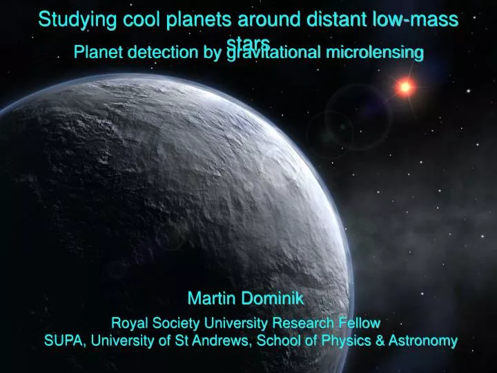
Studying cool planets around distant low-mass stars. Planet detection by gravitational microlensing. Martin Dominik. Royal Society University Research Fellow. SUPA, University of St Andrews, School of Physics & Astronomy. bending angle. 2 GM. α =. c 2 ξ. measurable at Solar limb: α = .

E N D
Studying cool planets around distant low-mass stars Planet detection by gravitational microlensing Martin Dominik Royal Society University Research Fellow SUPA, University of St Andrews, School of Physics & Astronomy
bending angle 2GM α = c2ξ measurable at Solar limb: α = 0.″85 suggested: measure during Solar eclipse Deflection of light by gravity (1911)
bending angle measurable at Solar limb: α = 1.″7 confirmed by measurement of stellar positions during Solar eclipse (Eddington 1919) Deflection of light by gravity (1915) 4GM α = c2ξ
S L Bending of starlight by stars (Gravitational microlensing) You are here
4GM bending angle α = c2ξ DS DL η ξ Deriving the gravitational lens equation side view I− L O S α α I+
4GM α = bending angle c2ξ I− η ξ I+ 1 y = x − x 1 x± = [y ± (y2+4)1/2] two images 2 The gravitational lens equation and its solutions side view angular Einstein radius ( ) 1/2 DS−DL 4GM θE = DLDS c2 ξ η y = x = (lens equation) DL θE DS θE
angular Einstein radius ( ) 1/2 DS−DL 4GM θE = DLDS c2 with ‘typical’ DS ~ 8.5 kpc and DL ~ 6.5 kpc θE ~ 600 (M/M☉)1/2 as μ dx± x± radial distortion tangential distortion dy y Image distortion and magnification observer’s view 1 x± = [y ± (y2+4)1/2] 2 lens equation relates radial coordinates, polar angle conserved x± dx± y2+2 A(y)= ∑ = total magnification y (y2+4)1/2 y dy ±
S L (t-t0)/tE y2+2 y(t) = [u02 + ()2]1/2 t − t0 tE=θE/μ A(y) = tE y (y2+4)1/2 tE~40(M/M☉)1/2days μ ~ 15 μasd-1 Microlensing light curves A[y(t)]defined by u0, t0, tE
Notes about gravitational lensing dated to 1912 on two pages of Einstein’s scratch notebook
ρ(DL) ∫ ∫ f(M) dM = 1 N →f(M) DL2 dDL dΩ dM M 1/2 ( ) DS−DL 4GM θE = DLDS c2 I 4πG 2πG ∫ τ = DS2ρx(1-x) dx = DS2ρ c2 3c2 0 M☉ DS ~ 8 kpc, Galactic disk ρ = 0.1 (pc)3 Microlensing optical depth quantify alignment by defining optical depthτ= probability that given source star is inside Einstein circle u < 1 ⇔ A > 3/√5 ≈ 1.34 corresponds to brightening in excess of 34% Solid angle of sky covered by NL Einstein circles NLπθE2 (neglect overlap) with mass volume density ρ(DL) and mass spectrum f(M) for ρ = const., x = DL/DS τ ~ 6 × 10⁻⁷ (Galactic disk) 35% disk, 65% bulge τ ~ 2 × 10⁻⁶ (total)
π <te> = tE 2 π (unit circle: area π, width 2, average length ) 2 τ Γ = NS = 2 × 10⁻⁵NS (yr)-1 <te> for 1000 events per year monitor NS ~ 5 × 10⁷ stars ~ 85 ongoing events at any time (Note: target observability shows seasonal variation) Microlensing surveys are a major data processing venture 1936: no computers 1965: computers not powerful enough Microlensing event rate event time-scale tE ~ 20 days during tE, source star moves on the sky by θE average duration of ‘event’ with A > 1.34 event rate
MACHO LMC#1 First reported microlensing event Nature 365, 621 (October 1993)
Optical Gravitational Lensing Experiment 1.3m Warsaw Telescope, Las Campanas (Chile) Current microlensing surveys (2007) 1.8m MOA Telescope, Mt John (New Zealand) daily monitor ≳ 100 million stars, τ ~ 10-6 for microlensing event → ~1000 events alerted per year
angular radius θ= RL/DL vs. angular Einstein radius ( ) 1/2 DS−DL 4GM θE = DLDS c2 of intervening object θ ≪ θE : lensing (brightening) θ ≫ θE : eclipse (dimming) Lensing or eclipse ? Condition for eclipse: foreground object occults the lensing images of the background object foreground object occults the background object Lensing regime: DL/DS ≈ 1/2, region broadens with increasing DS Eclipse regime: DS−DL ≫DL or DS ≫DL eclipsing planets around observed (source) stars microlensing planets around lens stars eclipsing stellar binaries Consequences: Text Prediction from data prior to first caustic peak
Microlensing detects planets around lens stars Host stars are selected by means of chance alignment Their mass distribution is related to stellar mass function Stellar mass probed by microlensing Microlensing prefers detecting planets around red-dwarf stars Which host stars?
x y = x− lens equation (2D) for single point-mass lens |x|2 θ β x = y = two-dimensional position angles β (source) and θ (image) θE θE ( ) 1/2 DS−DL 4GM θE = angular Einstein radius DLDS c2 ∑mi = 1 total mass M, i-th object with mass fraction mi at x(i), x − x(i) y = x− ∑mi |x − x(i)|2 Multiple point-mass lens in weak-field limit, superposition of deflection terms, but not of light curves
δ = d θE angular separation q = m2/m1 m2 = 1 − m1 mass ratio 1 q m1 = m2 = 1+q 1+q ( ) ( ) 1 q x(1) = d, 0 x(2) = −d, 0 in centre-of-mass system: 1+q 1+q q 1 x1 − d x1 + d 1 q 1+q 1+q y1= x1− − 1+q 1+q ( ) 2 q ( ) 1 2 x1 − d + x22 x1 + d + x22 1+q 1+q x2 x2 1 q y2= x2− − 1+q 1+q ( ) 2 q ( ) 1 2 x1 − d + x22 x1 + d + x22 1+q 1+q The binary point-mass lens completely characterized by two dimensionless parameters (d,q) time-scale of planetary deviations ≪orbital period solving for (x1,x2) leads to 5th-order complex polynomial either 3 or 5 images
∂y A(y) = ∑ ||-1 det () magnification (xj) ∂x j ∂y for det () (xj) = 0 for at least one j A(y) → ∞ ∂x ∂y det () caustics {yc = y(xc) |} (xc) = 0 ∂x point lens: critical points at x = 1 (Einstein circle), map to y = 0 (point caustic at position of lens) 3 topologies for a binary lens “resonance” at d ~ 1 Magnification and caustics
for q ≪ 1: two-scale problem lens star produces 2 images if planet close to one of these, it creates a further split maximal effect if lens star creates image near the planet tidal field of the star creates extended ‘planetary caustic’ there is also a ‘central caustic’ close to the lens star for d ~ 1, both merge into a single caustic d[1] planet-star separation in units of stellar angular Einstein radius position of planetary caustic (fulfills lens equation) 1 D = d[1]− d[1] inside Einstein circle (|D| < 1) for (√5−1)/2 < d[1] < (√5+1)/2 (“lensing zone”) green shades: brighter shading levels: more than 1%, 2%, 5%, 10% blue shades: dimmer Planetary-regime binary-lens caustics and excess magnification q = 10-2 red: caustics
Caustics and excess magnification (II) q = 10-2 q = 10-3
q = 10-2 q = 10-3 q = 10-4 light curve determined by 1D cut through 2D magnification map for event with (u0,t0,tE), only a fraction of all trajectory angles lead to detectable signal detection efficiency ε (d,q; u0,t0,tE) = P ( detectable signal in event (u0,t0,tE) | planet (d,q) ) Caustics and excess magnification (III) Detection efficiency
ρ✶ = θ✶/θE = 0.025 (giant R✶ ~ 15 R☉) Planetary deviations tE = 20 d tE = 20 d wide close [d] [d] q = 10-2 q = 10-3 q = 10-4
Planetary signals Linear size of deviation regions scale with q1/2 (planetary caustic) or q (central caustic) For point-like sources, both signal duration and probability scale with this factor Signal amplitude limited by finite angular source size θ✶ main-sequence star R✶ ~ 1 R☉ vs giant R✶ ~ 15 R☉ tE = 20 d planetary caustic tE = 20 d central caustic