Structural Decomposition Methods for Constraint Solving and Optimization

1. Please do not distribute beyond MERS group Structural Decomposition Methods for Constraint Solving and Optimization Martin Sachenbacher February 2003

2. Outline • Decomposition-based Constraint Solving • Tree Decompositions • Hypertree Decompositions • Solving Acyclic Constraint Networks • Decomposition-based Optimization • Dynamic Programming • Generalized OCSPs involving State Variables • Demo of Prototype • Decomposition vs. other Solving Methods • Conditioning-based Methods • Conflict-directed Methods

3. Outline • Decomposition-based Constraint Solving • Tree Decompositions • Hypertree Decompositions • Solving Acyclic Constraint Networks • Decomposition-based Optimization • Dynamic Programming • Generalized OCSPs involving State Variables • Demo of Prototype • Decomposition vs. other Solving Methods • Conditioning-based Methods • Conflict-directed Methods

4. Constraint Satisfaction Problems • Domains dom(vi) • Variables V = v1, v2, …, vn • Constraints R = r1, r2, …, rm • Tasks • Find a solution • Find all solutions

5. Methods for Solving CSPs • Generate-and-test • Backtracking • … “Guessing” • Truth Maintenance • Kernels • … • Analytic Reduction “Decomposition” “Conflicts”

6. Example r(E,B) E r(E,D) r(E,C) {1,2} 1 22 1 1 22 1 1 21 32 12 3   {1,2} {1,2,3}  D  C r(B,C) 1 22 1  {1,2} {1,2}  A B r(D,A) r(A,B) 1 22 1 1 22 1

7. Example • Eliminate Variable E r(E,B) E r(E,D) r(E,C) {1,2} 1 22 1 1 22 1 1 21 32 12 3   {1,2} {1,2,3}  D  C r(B,C) 1 22 1  {1,2} {1,2}  A B r(D,A) r(A,B) 1 22 1 1 22 1

8. Example r(B,C) r(D,B,C) 1 22 1 2 2 22 2 31 1 11 1 3 {1,2} {1,2,3} D C  {1,2} {1,2}  A B r(D,A) r(A,B) 1 22 1 1 22 1

9. Example (continued) • Eliminate variable D r(B,C) r(D,B,C) 1 22 1 2 2 22 2 31 1 11 1 3 {1,2} {1,2,3} D C  {1,2} {1,2}  A B r(D,A) r(A,B) 1 22 1 1 22 1

10. Example (continued) • Eliminate variable C r(A,B,C) r(A,B) 1 2 21 2 32 1 12 1 3 1 22 1 {1,2,3} C {1,2} {1,2} A B

11. Example (continued) • Eliminate variable B r(A,B) 1 22 1 {1,2} {1,2} A B

12. Example (continued) • Non-empty: Satisfiable! r(A) Backtrack-free 12 Extend “backwards”to find solutions {1,2} A

13. Idea of Decomposition • Computational Steps: Join, Project Var A: r(A) Var B: r(B,A) r(A,B) Var C: r(C,B) r(A,B,C) Var D: r(D,A) r(B,C,D) Var E: r(E,D) r(E,B) r(E,C)

14. Idea of Decomposition • Computational Scheme (acyclic) r(A) r(B,A) ⋈ r(A,B) r(C,B) ⋈ r(A,B,C) r(D,A) ⋈ r(B,C,D) r(E,D) ⋈ r(E,B) ⋈ r(E,C)

15. Idea of Decomposition • Alternative Scheme for the Example r(E,B) r(E,D) ⋈ r(B,D) r(E,C) ⋈ r(B,C) r(A,B) ⋈ r(A,D)

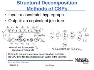
16. Tree Decompositions • A tree decomposition of a graph is a triple (T,,) where T=(N,E) is a tree,  and  are labeling functions associating with each node n  N two sets (n)  V, (n)  R such that: • For each rj  R, there is at least one n  N such that rj  (n) and scope(rj)  (n) (“covering”) • For each variable vi  V, the set {n  N | vi  (n)} induces a connected subtree of T (“connectedness”) • The tree-width of a tree decomposition is defined as max(|(n)|), n  N.

17. Tree Decompositions • Comparing Tree Decompositions for the Example R(A) Tree-Width 4 R(E,B) R(B,A) ⋈ R(A,B) R(E,C) ⋈ R(B,C) R(C,B) ⋈ R(A,B,C) R(E,D) ⋈ R(B,D) Tree-Width 3 R(D,A) ⋈ R(B,C,D) R(A,B) ⋈ R(A,D) R(E,D) ⋈ R(E,B) ⋈ R(E,C)

18. Structural Decomposition Methods • Biconnected Components [Freuder ’85] • Treewidth [Robertson and Seymour ’86] • Tree Clustering [Dechter Pearl ’89] • Cycle Cutset [Dechter ’92] • Bucket Elimination [Dechter ‘97] • Tree Clustering with Minimization [Faltings ’99] • Hinge Decompositions [Gyssens and Paredaens ’84] • Hypertree Decompositions [Gottlob et al. ’99]

19. Tree Clustering • Example A B C D E F

20. Tree Clustering • Step 1: Select Variable Ordering A B C D E F

21. Tree Clustering • Step 2: Make graph chordal (connect non-adjacent parents) A A B B C C D E F

22. Tree Clustering • Step 3: Identify maximal cliques A B C D E F

23. Tree Clustering • Step 4: Form Dual Graph using Cliques as Nodes A,B,C,E E B,C,E D,E D,E,F B,C,D,E

24. Tree Clustering • Step 5: Remove Redundant Arcs Tree-Width 4 A,B,C,E (E) B,C,E D,E D,E,F B,C,D,E

25. Tree Clustering • Alternative variable order F,E,D,C,B,A produces Tree-Width 3 F,D D B,C,D B,C (B) A,B,C B,A A,B,E

26. Decomposing Hypergraphs • Possible Approach: Turn hypergraph into primal/dual graph, then apply graph decomposition method • But: sub-optimal, conversion loses information • Idea [Gottlob 99]: Generalize decomposition to hypergraphs

27. Hypertree Decompositions • A triple (T,,) such that: • For each rj  R, there is at least one n  N such that scope(rj)  (n) (“covering”) • For each variable vi  V, the set {n  N | vi  (n)} induces a connected subtree of T (“connectedness”) • For each n  N, (n)  scope((n)) • For each n  N, scope((n))  (Tn)  (n), where Tn is the subtree of T rooted at n • The hypertree-width of a hypertree decomposition is defined as max(|(n)|), nN.

28. Tree-Width vs. Hypertree-Width • Class of CSPs with bounded HT-width subsumes class of CSPs with bounded tree-width ([Gottlob 00]) • Determining the HT-width of a CSP is NP-complete • For each fixed k, it can be determined in polynomial time whether the HT-width of a CSP is  k

29. Game Characterization: Tree-Width • Robber and k Cops • Cops want to capture the Robber • Each Cop controls a node of the graph • At any time, Robber and Cops can move to neighboring nodes • Robber tries to escape, but must avoid nodes controlled by Cops

30. Playing the Game q b a d g c f e p h j l i k o n m

31. First Move of the Cops q b a d g c f e p h j l i k o n m

32. Shrinking the Space q b a d g c f e p h j l i k o n m

33. The Capture q b a d g c f e p h j l i k o n m

34. Game Characterization: HT-Width • Cops are now on the edges • Cop controls all the nodes of an edge simultaneously

35. Playing the Game V P R S X Y T Z U W

36. First Move of the Cops V P R S X Y T Z U W

37. Shrinking the Space V P R S X Y T Z U W

38. The Capture V P R S X Y T Z U W

39. Different Robber’s Choice V P R S X Y T Z U W

40. The Capture V P R S X Y T Z U W

41. Strategies and Decompositions • Theorem: A hypergraph has hypertree-width  k iff k Cops have a winning strategy • Winning strategies correspond to decompositions and vice versa

42. First Move of the Cops a(S,X,T,R) ⋈ b(S,Y,U,P) V P R S X Y T Z U W

43. Possible Choice for the Robber a(S,X,T,R) ⋈ b(S,Y,U,P) V P R S X Y T Z U W

44. The Capture a(S,X,T,R) ⋈ b(S,Y,U,P) c(R,P,V,R) V P R S X Y T Z U W

45. Alternative Choice for the Robber a(S,X,T,R) ⋈ b(S,Y,U,P) c(R,P,V,R) V P R S X Y T Z U W

46. Shrinking the Space a(S,X,T,R) ⋈ b(S,Y,U,P) c(R,P,V,R) d(X,Y) ⋈ e(T,Z,U) V P R S X Y T Z U W

47. The Capture a(S,X,T,R) ⋈ b(S,Y,U,P) c(R,P,V,R) d(X,Y) ⋈ e(T,Z,U) V P R S d(X,Y) ⋈ f(W,X,Z) X Y T Z U W

48. Decomposition a(S,X,T,R) ⋈ b(S,Y,U,P) HT-Width 2 c(R,P,V,R) d(X,Y) ⋈ e(T,Z,U) d(X,Y) ⋈ f(W,X,Z)

49. Decomposition-based CSP Solving • Turn CSP into equivalent acyclic instance • Solve equivalent acyclic instance (polynomial in width) W(E,C) R(A,B) ⋈ S(D,A) U(E,D) T(B,C) T(B,C) ⋈ U(E,D) V(E,B) “Compilation” S(D,A) R(A,B) V(E,B) W(E,C)

50. Solving Acyclic CSPs • Bottom-Up Phase • Consistency check • Top-Down Phase • Solution extraction • Polynomial complexity • Highly parallelizable