Download

1 / 30
300 likes | 485 Views
Modelling Longitudinal Biomarkers of Disease Progression (Natural History of Prostate Cancer). Donatello Telesca Stochastic Modeling Preliminary Exam. Preview. Prostate Cancer Background Natural History Models Modeling Different Views A case study (BLSA)

E N D
Modelling Longitudinal Biomarkers of Disease Progression (Natural History of Prostate Cancer) Donatello Telesca Stochastic Modeling Preliminary Exam
Preview • Prostate Cancer Background • Natural History Models • Modeling Different Views • A case study (BLSA) • Model Assessment and Conclusions
Prostate Cancer • Most commonly diagnosed form of cancer in USA. • Usually diagnosed in men over 55 and slow growing. • Second most common cause of cancer death in American men (after lung cancer ) • The prostate gland plays a role in the male urinary and reproductive systems.
Natural History of Prostate Cancer Clinical Stage (Size and Extent of the tumor) Histologic Grade (Cell differentiation) Local Metastasis Gleason score 1 Gleason score 5
Natural History Models • Natural history models aim to chart the progression of a disease. • They provide critical information about the early stages of a disease. • They provide recommendations for cancer screening and detection. • The challenge is related to the latency of the main events comprising disease progression. • They usually rely on the availability of a biomarker associated to the presence and progression of the disease.
PSA and Prostate Cancer • PSA (Prostate Specific Antigen) is a protein produced by the prostate gland to keep the semen in a liquid state. Disease Onset Cancer PSA Level Normal Puberty AGE
Different Views on Disease Progression • Prostate adenocarcinomas have a different natures directly from onset. Some are more aggressive (Low cell differentiation), others are less aggressive (Good cell differentiation). • Prostate adenocarcinomas have a progressive nature. They start out as well differentiated tumor cells and they progress with time to more aggressive forms, with poorly differentiated tumor cells.
A model with no grade progression TM : Metastasis (Advanced) TM : Metastasis (Local) High Grade Low Grade Log(PSA+α) Tc : Clinical Diagnosis T0 : Onset Time AGE
PSA Trajectories Subject level Population level
Disease Onset Hazard Cumulative Hazard Density
Time to Diagnosis and Metastasis Time to Metastasis Hazard Cumulative Hazard Monotonicity Time to Clinical Diagnosis Hazard Cumulative Hazard
A causal diagram of grade progression Onset Grade trans. t0 tG PSA tC tM Metastasis Diagnosis
A model with grade progression tg : Grade transition Log(PSA + α) tM : Metastasis t0 : Onset tc : Diagnosis AGE
PSA Trajectories Subject level Population level
Grade Transition Hazard t0
Time to Metastasis Hazard Monotonicity:
Likelihood yi: log(PSA + const) for individual i θ : parameter vector x : stage(1=local, 2=metastasis) Local stage Advanced Stage
Bayesian Estimation POSTERIOR Chained data augmentation • i) Given (t0(k-1), tM(k-1)) , θ(k) ~ π(θ|y, tc, x, t0(k-1) ,tM(k-1)); • Given θ(k) , (t0(k-1) , tM(k-1))~ π(θ|y, tc, x, t0(k-1) ,tM(k-1) ); • Iterate (i), (ii).
Dealing with constrained parameter spaces (Example) Growth rates full conditional: With constraints: • bi0 ~ bi0|yi,θ(-bi0) • bi1 ~ bi1|yi,θ(-bi1) in (bi1>-bi2) • bi2 ~ bi2|yi,θ(-bi2) in (bi2>-bi1) • bi3 ~ bi3|yi,θ(-bi3) in (bi3>-(bi1+bi2)) bi2=-bi1 bi3 = -(bi1+bi2) bi2 bi1+bi2 bi1 bi3
Model Fit Comparison Subject with local disease and high grade Progressive grade No grade progression Log(PSA + 0,03) Log(PSA + 0,03) Age Age
Model Fit Comparison Subject with advanced disease and high grade Progressive grade No grade progression Log(PSA + 0,03) Log(PSA + 0,03) Age Age
Model Fit Comparison Subject with local disease and low grade Progressive grade No grade progression Log(PSA + 0,03) Log(PSA + 0,03) Age Age
Posterior Predictive Assessment Posterior predictive distributions for transition times and median predictive PSA trajectories, assuming no grade progression . (High GS) Log(PSA + 0.03) (Low GS) Density 4ng/ml Age
Posterior Predictive Assessment Posterior predictive distributions for transition times and median predictive PSA trajectory, assuming grade progression . Log(PSA + 0.03) Density 4ng/ml Age
Model Assessment M1: No grade progression M2: Grade progression ● Bayes Factor → Strong evidence against M2
CPO Analysis ● No Grade progression ● Grade progression o Log( CPO ) = Log( f(yi, tci, xi|y-i, tc,-i ,x-i) ) Log(CPO) Subject
Concluding • We proposed a way to translate scientific hypotheses about the progression of prostate cancer into a statistical model for the disease main biomarker (PSA). • The BLSA data provides evidence in favor of the hypothesis of no grade progression as opposed to that of grade progression. • Limitations of this approach : - Difficult validation of the hazard models for the latent transition times. - Prior sensitivity. • Extensions may consider : - Misclassified diagnosis of the normal subjects. - Non-parametric formulation of the problem.
Acknowledgements • Julian Besag • Lourdes Inoue • Stat518(2005): Congley, Haoyuan, Liang, Nate, Yanming.
Adaptive Slice Sampling (R.M. Neal, 2000) f(x0) S y ~ U[0,f(x0)] x1 ~ U(S) x0