Download
1 / 44
440 likes | 569 Views
More Chapter 4. Sufficient statistics. The Poisson and the exponential can be summarized by (n, ). So too can the normal with known variance Consider a statistic S(Y)

E N D
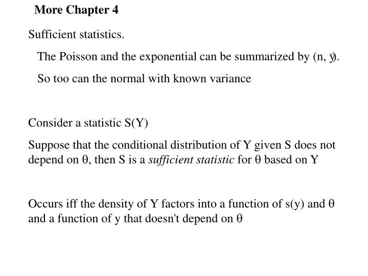
More Chapter 4 Sufficient statistics. The Poisson and the exponential can be summarized by (n, ). So too can the normal with known variance Consider a statistic S(Y) Suppose that the conditional distribution of Y given S does not depend on , then S is a sufficient statistic for based on Y Occurs iff the density of Y factors into a function of s(y) and and a function of y that doesn't depend on
Example. Exponential IExp() ~ Y E(Y) = Var(Y) = 2 Data y1,...,yn L() = -1 exp(-yj /) l() = -nlog() - yj / yj /n is sufficient
Approximate 100(1-2 )% CI for 0 Example. spring data
Note. Expected information
Example. Bernoulli Pr{Y = 1} = 1 - Pr{Y = 0} = 0 1 L() = ^yi (1 - )^(1-yi) = r(1 - )n-r l() = rlog() + (n-r)log(1-) r = yj R = Yj is sufficient for , as is R/n L() factors into a function of r and a constant
Score vector [ yj / - (n-yj )/(1-)] Observed information [yj /2 + (n-yj )/(1-)2 ] M.l.e.
Cauchy. ICau() f(y;) = 1/(1+(y-)2 ) E|Y| = Var(Y) = L() = 1/((1+(yj -)2 ) Many local maxima l() = -log(1+(yj -)2 ) J() = 2((1-(yj -)2 )/(1+(yj -)2 )2 I() = n/2
Uniform. f(u;) = 1/ 0 < u < = 0 otherwise L() = 1/n 0 < y1 ,..., yn < = 0 otherwise
l() becomes increasingly spikey E u() = -1 i() = -
Logistic regression. Challenger data Ibinomials Rj , mj , j
Likelihood ratio. Model includes dim() = p true (unknown) value 0 Likelihood ratio statistic
Justification. Multinormal result If Y ~ N (,) then (Y- )T -1(Y- ) ~ p2
Uses. Pr[W(0) cp(1-2 )] 1-2 Approx 100(1-2 )% confidence region
Example. exponential Spring data: 96 < <335 vs. asymp normal approx 64 < <273 kcycles
Prob-value/P-value. See (7.28) Choose T whose large values cast doubt on H0 Pr0(T tobs) Example. Spring data Exponential E(Y) = H0: = 100?
Nesting : p by 1 parameter of interest : q by 1 nuisance parameter Model with params (0, ) nested within(, ) Second model reduces to first when = 0
Example. Weibull params (,) exponential when = 1 How to examine H0 : = 1?
Challenger data. Logistic regression temperature x1 pressure x2 (0 , 1 , 2 ) = exp{}/(1+exp{}) = 0 + 1 x1 + 2 x2 linear predictor loglike l(0 , 1 , 2 ) = 0 rj + 1 rj x1j + 2 rj x2j - m log(1+exp{j }) Does pressure matter?
Model fit. Are labor times Weibull? Nest its model in a more general one Generalized gamma. Gamma for =1 Weibull for =1 Exponential for ==1
Likelihood results. max log likelihood: generalized gamma -250.65 gamma -251.12 Weibull -251.17 gamma vs. generalized gamma - 2 log like diff: 2(-250.65+251.12) = .94 P-value Pr0 (12 > .94) = Pr(|Z|>.969) = 2(.166) = .332
Chi-squared statistics. Pearson's chi-squared categories 1,...,k count of cases in category i: Yi Pr(case in i) = i 0 < i < 1 1ki =1 E(Yi ) = ni var(Yi ) = i(1 - i )n cov(Yi ,Yj ) = -ij n i j E.g. k=2 case cov(Y,n-Y) = -var(Y) = -n12 = { (1 ,...,k ): 1ki = 1, 0<1 ,...,k <1} dimension k-1
Reduced dimension possible? model i () dim() = p log like general model: 1k-1 yi log i + yk log[1-1 -...-k-1], 1k yi = n log like restricted model: l() = 1k-1 yi log i() + yk log[1-1()-...-k-1()]
likelihood ratio statistic: if restricted model true The statistic is sometimes written W = 2 Oi log(Oi /Ei ) (Oi - Ei )2/Ei
Example. Birth data. Poisson? Split into k=13 categories [0,7.5), [7.5,8.5),...[18.5,24] hours O(bserved) 6 3 3 8 ... E(xpected) 5.23 4.37 6.26 8.08 ... P = 4.39 P-value Pr(112 > 4.39) = .96
Two way contingency table. r rows and c columns n individuals Blood groups A, B, AB, O A, B antigens - substance causing body to produce antibodies group count model I model II O = 1 - A - B
Question. Rows and columns independent? W = 2 yij log nyij / yi.y.j with yi. = j yij ~ k-1-p2 = (r-1)c-1)2 with k=rc p=(r-1)+(c-1) P = (yij - yi. y.j /n)2 / (yi. y.j /n) ~ (r-1)(c-1)2
Model 1 W = 17.66 Pr(12> 17.66) = Pr(|Z| > 4.202) = 2.646E-05 P = 15.73 Pr(12> 15.73) = Pr(|Z| > 3.966) = 7.309E-05 k-1-p = 4-1-2 = 1 Model 2 W = 3.17 Pr(|Z| > 1.780) = .075 P = 2.82 Pr(|Z|>1.679) = .093
Incorrect model. True model g(y), fit f(y;)
Model selection. Various models: non-nested Ockham's razor. Prefer the simplest model
Formal criteria. Look for minimum
Example. Spring failure Model p AIC BIC M1 12 744.8* 769.9* M2 7 771.8 786.5 M3 2 827.8 831.2 M4 2 925.1 929.3 6 stress levels M1: Weibull - unconnected , at each stress level