Download
1 / 27
290 likes | 605 Views
Software Process Metrics. Sources: Roger S. Pressman, Software Engineering – A Practitioner’s Approach, 5 th Edition, ISBN 0-07-365578-3, McGraw-Hill, 2001 (Chapters 4 & 24)

E N D
Software Process Metrics • Sources: • Roger S. Pressman, Software Engineering – A Practitioner’s Approach, 5th Edition, ISBN 0-07-365578-3, McGraw-Hill, 2001 (Chapters 4 & 24) • Stephen H. Kan, Metrics and Models in Software Quality Engineering, 2nd Edition, ISBN 0-201-72915-6, Addison-Wesley, 2003
Measurement & Metrics • What is it? • Software process and product metrics are quantitative measures that enable software people to gain insight into the efficacy of the software process and the projects that are conducted using the process as a framework. • Who does it? • Software metrics are analyzed and assessed by software managers. • Why is it important? • If you don't measure, judgment can be based only on subjective evaluation. • What are the steps? • Begin by defining a limited set of process, project, and product measures that are easy to collect.
Measurement & Metrics – Cont.. • What is the work product? • A set of software metrics that provide insight into the process and understanding of the project. • How do I ensure that I've done it right? • By applying a consistent, yet simple measurement scheme that is never to be used to assess, reward, or punish individual performance.
Why do we Measure? • To characterize – to gain understanding of process, products, resources, and environments, and to establish baselines for future assessments • To evaluate – to determine status with respect to plans. • To predict – so that we can plan. • To improve – we gather information to help us identify road blocks, root causes, inefficiencies, and other opportunities for improving product quality and process performance.
A Good Manager Measures process process metrics project metrics measurement product metrics product What do we use as a basis? • size? • function?
Process Metrics • majority focus on quality achieved as a consequence of a repeatable or managed process • statistical SQA data • error categorization & analysis • defect removal efficiency • propagation from phase to phase • reuse data
Metrics Guidelines • Use common sense and organizational sensitivity when interpreting metrics data. • Provide regular feedback to the individuals and teams who have worked to collect measures and metrics. • Don’t use metrics to appraise individuals. • Work with practitioners and teams to set clear goals and metrics that will be used to achieve them. • Never use metrics to threaten individuals or teams. • Metrics data that indicate a problem area should not be considered “negative.” These data are merely an indicator for process improvement. • Don’t obsess on a single metric to the exclusion of other important metrics.
Failure Analysis Failure analysis works in the following manner: • All errors and defects are categorized by origin (e.g., flaw in specification, flaw in logic, nonconformance to standards). • The cost to correct each error and defect is recorded. • The number of errors and defects in each category is counted and ranked in descending order. • The overall cost of errors and defects in each category is computed. • Resultant data are analyzed to uncover the categories that result in highest cost to the organization. • Plans are developed to modify the process with the intent of eliminating (or reducing the frequency of) the class of errors and defects that is most costly.
Managing Variation • Because software process and the product it produces both are influenced by many parameters, metrics collected for one project or product will not be the same as similar metrics collected for another project. • How can we tell if improved (or degraded) metrics values that occur as consequence of improvement activities are having a quantitative impact? • How do we know whether we’re looking at a statistically valid trend or whether the “trend” is simply a result of statistical noise? • When are changes (either positive or negative) to a particular software metric meaningful? • A graphical technique called “control chart” is available for determining whether changes and variation in metrics data are meaningful.
Collecting Data • The Principal tasks are: • Designing the methods and obtaining the tools to support data collection and retention. • Obtaining and training staff for the data collection procedures. • Capturing and recording data for each process that is targeted for measurement. • Using defined forms and formats to supply the collected data to those who perform analyses. • Monitoring the execution (compliance) and performance of the activities for collecting and retaining data.
Process Performance Variation • Shewhart (1931) categorize sources of variation as follows: • Variation due to phenomena that are natural and inherent to the process and whose results are common to all measurement of a given attribute. • Variations that have assignable causes that could have been prevented. [total variation] = [common cause variation] + [assignable cause variation] • Common cause variation of process performance is characterized by a stable and consistent pattern of measured values over time (cf. figure below
Variations in process performance due to assignable causes have marked impacts on product characteristics and other measures of performance. • These impacts create significant changes in the patterns of variations, as illustrated in the figure below. These variations arise from events that are not part of the normal process.
Stability Concepts and Principles • A stable process is one that is in statistical control. • Sources of variability in stable process are due solely to common causes. • Variations due to assignable causes have been either removed and prevented from re-entering or incorporate as a permanent part of the process (if beneficial).
Testing for Stability • We need to know how variable the values are within the subgroup (samples) at each measurement point, and • We need to compare this to the variability that we observe from one subgroup to another. • Specifically we need to determine whether the variation over time is consistent with the variation that occurs within the subgroup and detect possible drift or shift from the central tendency • X-bar and R Charts for a process that is in control • The X-bar (top) shows the changes in averages • The R chart shows the observed dispersion in process performance across subgroups
Out-of-Control Process • The figure below shows a process that is out-of-control. • This is because the subgroup range exceeds its upper control limit (UCL) at t5.
Control Chart Basics • The basic layout is given below. • The Centerline (CL) is usually the observed process average. • The control limits (LCL and UCL) are ±3 standard deviation (σ). Other measures could be used.
Detecting Instability and out-of-control situations • Testing for instability is done by examining the control charts for patterns and values falling outside the control limits suggest assignable causes exist.
Several tests are available for detecting unusual patterns and nonrandom behavior. The Western Electric Handbook cites four that are effective [Western Electric 1958; Wheeler 1992. 1995]. Figure above illustrates the following four tests: • Test I: A single point falls outside the 3-sigma control limits. • Test 2: At least two out of three successive values fall on the same side of, and more than two sigma units away from. the centerline. • Test 3: At least four out of five successive values fall on the same side of, and more than one sigma unit away from. the centerline. • Test 4: At least eight successive values fall on the same side of the centerline. • Tests 2. 3. and 4 are called run tests and are based on the presumptions that the distribution of the inherent, natural variation is symmetric about the mean, that the data are plotted in time sequence. and that successive observed values are statistically independent.
Example: • Consider a software organization that collects the process metric, errors uncovered per review hour, Er. • Over 15 months, the organization collected Er for 20 small projects in the same general software development domain. • The resultant values for Er are represented in Figure 3.1. In the figure, Er varies from a low of 1.2 for project 3 to a high of 5.9 for project 17. • To improve the effectiveness of the reviews, the software organization can provide training and mentoring to all project team members.
The mR Control Chart – Metric data for errors uncovered per review hour Figure 3.1
moving range (mR) control chart • The procedure required to develop a moving range (mR) is: 1. Calculate the moving ranges: the absolute value of the successive differences between each pair of data points. Plot these moving ranges on your chart. 2. Calculate the mean of the moving ranges . . . plot this ("mR bar") as the center line on your chart. 3. Multiply the mean by 3.268. Plot this line as the upper control limit [UCL]. This line is three standard deviations above the mean. • Using the data represented in figure 3.1 and the steps above, mR control chart shown in figure 3.2 is developed. • The mR bar (mean) value for the moving range data is 1.71. • The upper control limit is 5.58 • A simple question is asked in order to determine whether the process metrics dispersion is stable – Are all the moving range values inside UCL? Yes for our example. Hence, the metrics dispersion is stable.
Moving range control chart Figure 3.2
Individual control chart • The individual control chart is developed in the following manner: • Plot individual metrics values as shown in Figure 3.1. • Compute the average value, Am, for the metrics values. • Multiply the mean of the mR values (the mR bar) by 2.660 and add Am computed in step 2. This results in the upper natural process limit (UNPL). Plot the UNPL. • Multiply the mean of the mR values (the mR bar) by 2.660 and subtract this amount from Am computed in step 2. This results in the lower natural process limit (LNPL). Plot the LNPL. If the LNPL is less than 0.0, it need not be plotted unless the metric being evaluated takes on values that are less than 0.0. • Compute a standard deviation as (UNPL - Am)/3. Plot lines one and two standard deviations above and below Am. If any of the standard deviation lines is less than 0.0, it need not be plotted unless the metric being evaluated takes on values that are less than 0.0. • Applying these steps to the data represented in Figure 3.1 - we derive an individual control chart as shown in Figure 3.3
Individual Control chart Figure 3.3
Zone Rules • Four criteria, called zone rules, that may be used to evaluate whether the changes represented by the metrics indicate a process that is in control or out of control. • If any of the following conditions is true, the metrics data indicate a process that is out of control: • A single metrics value lies outside the UNPL. • Two out of three successive metrics values lie more than two standard deviations away from Am. • Four out of five successive metrics values lie more than one standard deviation away from Am. • Eight consecutive metrics values lie on one side of Am.