Download
1 / 31
310 likes | 541 Views
On the modeling and simulation of large-scale systems. Venkataramanan (Ragu) Balakrishnan School of ECE, Purdue University Joint work with Stephen Cauley, Jitesh Jain, Hong Li, Cheng-Kok Koh (Purdue) and M. P. Anantram (NASA). Basic ideas. Many engineering system models are of a large scale

E N D
On the modeling and simulation of large-scale systems Venkataramanan (Ragu) Balakrishnan School of ECE, Purdue University Joint work with Stephen Cauley, Jitesh Jain, Hong Li, Cheng-Kok Koh (Purdue) and M. P. Anantram (NASA)
Basic ideas • Many engineering system models are of a large scale • However, most interactions are local • Problems: • Modeling that captures locality • Exploitation in simulation
Outline • One modeling example • One simulation example
VLSI interconnect modeling • Interconnects are relatively long wires connecting circuit elements • To account for distributed effects: • Wires broken into short segments • Segments further subdivided into filaments (if necessary) • Surfaces subdivided in panels (if necessary) • Result, a large-scale RLC model
The interconnect model • Model parameterized by very large matrices (size 104 or higher) • obtained by inverting , the potential matrix, which maps charges to voltages • obtained directly from magnetic vector potential; entries are self- and mutual-inductances
Model structure • is diagonal • is approximated as sparse • is dense, but inverse is approximately sparse • Sparsity structure:
Model extraction • Entries of and obtained via CAD tools • and approx. sparse • Modeling issues: • Detecting approx. sparsity pattern and • Approximating and s.t. inverses are sparse, with • Parameterization of and • Efficient computation (say matrix-vector multiplies) with and
Some answers • Interconnect modeling is part of an engineering design flow • Partial answers available from design stage; e.g., sparsity pattern in and • Focus on approximation problem • Begin with simple case: Given , find with tridiagonal
Tridiagonal case • Key result: Suppose with tridiagonal. Under mild conditions: • Result from late 1950s • Parameters computed as • Only tridiagonal entries of needed
Tridiagonal band-matching • Given : • Construct from tridiag entries of : • Define:
Tridiagonal band-matching Then: • is tridiagonal • can be computed in • Products and computable in • We have • Optimality? • minimizes Kullback-Leibler distance:
General case • Given seek with block-banded ( blocks, block-size , block bandwidth ) • “Band-matching” gives approximant s.t: • is block-banded, with • In-band entries of and match • is an “optimal” approximant • specified by parameters, requiring computation • Products and can be computed in
Further issues • Numerical stability: • Tridiagonal case: • Parameterization with ill-conditioned • Instead of , use ratios , … • Extension possible to block-tridiagonal case • Simulation without explicit computation of parameters • Structure of matrices whose inverses have more general sparsity patterns
Outline • One modeling example • One simulation example
Nano-scale simulation • Problem: Determine and evaluate dynamic behavior of the device • Macro-level simulation techniques of unacceptable accuracy • Need quantum mechanical modeling
2D Simulation of Nanotransistors Nonequilibrium Green’s Function approach: • Form Hamiltonian • Write out the equations of motion for the retarded ( ) and less-than ( ) Green’s functions • Solve for density of states and charge density
Mathematical Formulation Need diagonal entries of and • , • A is block-tridiagonal: , • Typical values:
Current state of the art • Marching algorithm due to Anant et al • Computational complexity: • Memory consumption: • For a problem of size this translates to 16GB( ) and 32GB ( ) of memory! [Anant02] - A. Svizhenko, M. P. Anantram, T. R. Govindan, B. Biegel, and R. Venugopal. Two-dimensional quantum mechanical modeling of nanotransistors. Journal of Applied Physics, 91(4):2343–2354, 2002.
New divide and conquer algorithm • Comparable computational efficiency: • Similar numerical conditioning • Significantly reduced memory requirements: allowing for large problems to be run on a single desktop computer • Flexibility to distribute computation across multiple processors, due to its inherent ability to be parallelized
Approach • Compute inverse of block-tridiagonal matrices • Adjust for “low rank” correction term (Procedure can be continued recursively) Low rank Correction terms
Inverting Computing and :
Applying low-rank corrections • Updating first block-row and last block-column too costly • Instead, accumulate low-rank maps that underlie updates
Matrix maps • For combining sub-problems, and for computing diagonal entries of inverse • Maps depend on corner blocks of sub-problem solutions
2 3 4 Parallel Implementation • Separate problem into . divisions • Data passed to first division is: 1
I II III IV III I IV II Parallel Implementation • Each CPU only modifies its matrix maps • Information exchanged at each combining step: Few . matrices
Single computer implementation • Problem separated into divisions • First pass: Divisions solved one after the other, and matrix maps computed • Second pass: Divisions re-solved for first block-row and last block-column of the inverses, and matrix maps applied to get final answer
Computation • There are divisions; computation of first block-row and block column of each division requires computation • There are combining stages. During each stage, for each division, map update requires computation • Total: • Single computer: • CPUs:
Memory • There are divisions; storage of first block-row and block column of each division requires memory • For each division, maps require storage • Total: • Single computer: • CPUs:
** Single Computer (min) Multi-processor (min) Results* * * All results are reported for the Retarded Green’s Function (Gr) ** as compared to [Anant02] with Nx = 100
Conclusions • Mathematical problems underlying applications presented well-studied • Examples of recent work: • Hierarchical (H) matrices (Hackbush et al.) • Nested dissection (Darve et al.) • Much of recent work in general settings • Presented work closer to application end; potential to exploit problem-specific information at the expense of generality