Download
1 / 23
230 likes | 351 Views
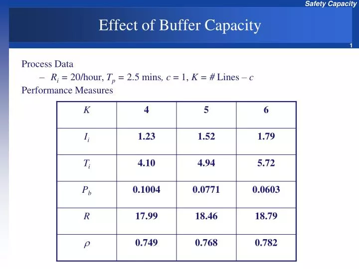
Effect of Buffer Capacity. Process Data R i = 20/hour, T p = 2.5 mins , c = 1, K = # Lines – c Performance Measures. Economics of Capacity Decisions. Cost of Lost Business C b $ / customer Increases with competition Cost of Buffer Capacity C k $/unit/unit time

E N D
Effect of Buffer Capacity • Process Data • Ri = 20/hour, Tp = 2.5 mins, c = 1, K = # Lines – c • Performance Measures
Economics of Capacity Decisions • Cost of Lost Business Cb • $ / customer • Increases with competition • Cost of Buffer Capacity Ck • $/unit/unit time • Cost of Waiting Cw • $ /customer/unit time • Increases with competition • Cost of Processing Cs • $ /server/unit time • Increases with 1/ Tp • Tradeoff: Choose c, Tp, K • Minimize Total Cost/unit time = Cb Ri Pb + Ck K + Cw I (or Ii) + c Cs
Optimal Buffer Capacity • Cost Data • Cost of telephone line = $5/hour, Cost of server = $20/hour, Margin lost = $100/call, Waiting cost = $2/customer/minute • Effect of Buffer Capacity on Total Cost
Performance Variability • Effect of Variability • Average versus Actual Flow time • Time Guarantee • Promise • Service Level • P(Actual Time Time Guarantee) • Safety Time • Time Guarantee – Average Time • Probability Distribution of Actual Flow Time • P(Actual Time t) = 1 – EXP(- t / T)
Effect of Blocking and Abandonment Blocking: the buffer is full = new arrivals are turned away Abandonment: the customers may leave the process before being served Proportion blocked Pb Proportion abandoning Pa
Net Rate: Ri(1- Pb)(1- Pa)Throughput Rate:R=min[Ri(1- Pb)(1- Pa),Rp] Effect of Blocking and Abandonment
Example 8.8 - DesiCom Call Center • Arrival Rate Ri= 20 per hour=0.33 per min • Processing time Tp =2.5 minutes (24/hr) • Number of servers c=1 • Buffer capacity K=5 • Probability of blocking Pb=0.0771 • Average number of calls on hold Ii=1.52 • Average waiting time in queue Ti=4.94 min • Average total time in the system T=7.44 min • Average total number of customers in the system I=2.29
Example 8.8 - DesiCom Call Center • Throughput Rate • R=min[Ri(1- Pb),Rp]= min[20*(1-0.0771),24] • R=18.46 calls/hour • Server utilization: • R/ Rp=18.46/24=0.769
Capacity Investment Decisions • The Economics of Buffer Capacity • Cost of servers wages =$20/hour • Cost of leasing a telephone line=$5 per line per hour • Cost of lost contribution margin =$100 per blocked call • Cost of waiting by callers on hold =$2 per minute per customer • Total Operating Cost is $386.6/hour
Example 8.10 - The Economics of Processing Capacity • The number of line is fixed: n=6 • The buffer capacity K=6-c
Variability in Process Performance • Why considering the average queue length and waiting time as performance measures may not be sufficient? • Average waiting time includes both customers with very long wait and customers with short or no wait. • We would like to look at the entire probability distribution of the waiting time across all customers. • Thus we need to focus on the upper tail of the probability distribution of the waiting time, not just its average value.
Example 8.11 - WalCo Drugs • One pharmacist, Dave • Average of 20 customers per hour • Dave takes Average of 2.5 min to fill prescription • Process rate 24 per hour • Assume exponentially distributed interarrival and processing time; we have single phase, single server exponential model • Average total process is; • T = 1/(Rp – Ri)= 1/(24 -20) = 0.25 or 15 min
Example 8.11 - Probability distribution of the actual time customer spends in process (obtained by simulation)
Example 8.11 - Probability Distribution Analysis • 65% of customers will spend 15 min or less in process • 95% of customers are served within 40 min • 5% of customers are the ones who will bitterly complain. Imagine if they new that the average customer spends 15 min in the system. • 35% may experience delays longer than Average T,15min
Service Promise:Tduedate ,Service Level & Safety Time • SL; The probability of fulfilling the stated promise. The Firm will set the SL and calculate the Tduedate from the probability distribution of the total time in process (T). • Safety time is the time margin that we should allow over and above the expected time to deliver service in order to ensure that we will be able to meet the required date with high probability • Tduedate = T+Tsafety • Prob(Total time in process<=Tduedate) = SL • Larger SL results in grater probability of fulfilling the promise.
Due Date Quotation • Due Date Quotation is the practice of promising a time frame within which the product will be delivered. • We know that in single-phase single server service process; the Actual total time a customer spends in the process is exponentially distributed with mean T. • SL = Prob(Total time in process<=Tduedate) = 1 – EXP( - Tduedate /T) • Which is the fraction of customers who will no longer be delayed more than promised. • Tduedate = -T ln(1 – SL)
Example 8.12 - WalCo Drug • WalCo has set SL = 0.95 • Assuming total time for customers is exponential • Tduedate = -T ln(1 – SL) • Tduedate = -T ln(0.05) = 3T • Flow time for 95 percentile of exponential distribution is three times the average T • Tduedate = 3 * 15 = 45 • 95% of customers will get served within 45 min • Tduedate = T+Tsafety • Tsafety = 45 – 15 = 30 min • 30 min is the extra margin that WalCo should allow as protection against variability
Relating Utilization and Safety Time: Safety Time Vs. Capacity Utilization • Capacity utilization ρ 60 % 70% 80% 90% • Waiting time Ti 1.5Tp 2.33Tp 4Tp 9Tp • Total flow time T= Ti + Tp 2.5Tp 3.33Tp 5Tp 10Tp • Promised time Tduedate 7.7Tp 10Tp 15Tp 30Tp • Safety time Tsafety = Tduedate – T 5Tp 6.67Tp 10Tp 20Tp • Higher the utilization; Longer the promised time and Safety time • Safety Capacity decreases when capacity utilization increases • Larger safety capacity, the smaller safety time and therefore we can promise a shorter wait
Managing Customer Perceptions and Expectations • Uncertainty about the length of wait (Blind waits) makes customers more impatient. • Solution is Behavioral Strategies • Making the waiting customers comfortable • Creating distractions • Offering entertainment
Thank you • Questions?