Download
1 / 20
200 likes | 347 Views
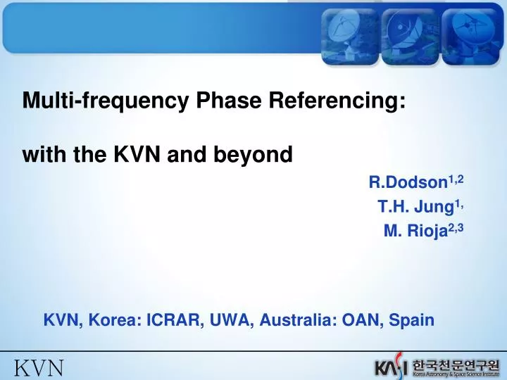
Multi-frequency Phase Referencing: with the KVN and beyond. R.Dodson 1,2 T.H. Jung 1, M. Rioja 2,3 KVN, Korea: ICRAR, UWA, Australia: OAN, Spain. Alternative Tropospheric Calibration in mm -VLBI. Conventional Phase referencing to a calibrator source ( requirements difficult to meet ).

E N D
Multi-frequency Phase Referencing:with the KVN and beyond R.Dodson1,2 T.H. Jung1, M. Rioja2,3 KVN, Korea: ICRAR, UWA, Australia: OAN, Spain
AlternativeTroposphericCalibrationin mm-VLBI Conventional Phase referencingto a calibratorsource (requirementsdifficulttomeet) • Observe at lowerband (e.g. 21.5 GHz) • Applytohigherband (e.g. 43 GHz) fast 43 43 GHz Different source Multi-frequency: phase ref. to a lowerfrequency Same source fast
Target Basics of new method: SOURCE/FREQ. phase referencing fast slow slow X A,GEO + A,TRO + STA,STR+nA High: A,GEO + A,TRO + STnA RRA,GEO + A,TRO + STnA) Low: High: R A,TRO- R *A,TRO= 0 A,XYZ- R *A,XYZ= 0, Antennaerrors cancel! - R*= (R-1/R) … slow slow RSTR+ 2c (D . A,shift)+ ST Frequency Phase Transfer
Basicsofnewmethod:SOURCE/FREQ. phasereferencing Introduce a SecondSource B R2c (D . B,shift)+ ION NST Same as for A Source/freq. referencedVisibilityphase: A,STR + 2c D (A,shift - B,shift)
Importantpoints • “Perfect” Tropospheric calibration • Non-integer ratio betweenfrequenciesproblematic (Introducesphasejumpsrelatedtophaseambiguities) • Frequency agility crucial: VLBA (switching); • Best simultaneous observations: KVN (Yebes-40m) • Direct Astrometric measurement of “core-shifts”, even • at the highest frequencies, > 43 GHz • Errors in station coordinates no problem (for cont. VLBI) …… 2π (nA - nB+ R(nA - nB))
KVN 3x 21m Antennas in S. Korea With 4 band simultaneous mm-wave receiver system: 22, 43, 86 & 129 GHz http://kvn-web.kasi.re.kr/en/en_obs_information.php
1st KVN 4-band Fringes (2012 April) KUS-KYS Fringe Phase (deg) 86GHz 43GHz 129GHz Fringe Amplitude (Jy) 22GHz IF13 IF14 IF15 IF16 IF1 IF2 IF3 IF4 IF5 IF6 IF7 IF8 IF9 IF10 IF11 IF12 16MHz x 16CH
Delay K-band Rate K13015a Jan 15, 2013
Delay Q-band Rate K13015a Jan 15, 2013
Delay W-band Rate K13015a Jan 15, 2013
Delay D-band Rate K13015a Jan 15, 2013
MFPR applied Visibility Phase @ Q-band (Rate Corrected) MFPR applied with K-band solint 0.1 Bad weather at Yonsei MFPR applied with K-band solint 0.3 K13015a: Jan 15, 2013
MFPR applied Visibility Phase @ W-band (Rate Corrected) MFPR applied with K-band solint 0.1 Low SNR at 22GHz Yonsei W-band v. high Tsys MFPR applied with K-band solint 0.3
MFPR applied Visibility Phase @ D-band (Rate Corrected) MFPR applied with K-band solint 0.1 Low SNR at 22GHz Poor temp. control (±6oC) MFPR applied with K-band solint 0.3
VLBA demonstrations • 86GHz (relative) phase referencing not first (Porcas&Rioja) but only practical Measured `core-shifts’ between 43&86 of <10μas Target is SiO maser alignment • 43GHz Absolute Astrometry 22 GHz conventional PR + 22/43GHz SFPR
VLBA demonstrations FPT: Sources track each other SFPR: Phases are at `zero’ FPT: Sources have common residuals Image at phase centre SFPR: Astrometrically corrected phases Offsets from centre are the position difference btw frequencies
Beyond KVN: Sim. mm-VLBI facilities VLBA has long baselines. KVN lacks these KVN uv-coverage: KAVA uv-coverage: Global uv-coverage: Potential to achieve~40μas with 2mm VLBI
Consequence of Adding KVN to VERA KVN And VERA Array Much greater sensitivity to low(er) surface brightness
Beyond SFPR: MFPR Can we find the corrections for ionosphere and instrumental terms in the data itself? Require ΔTEC → 0 In principle measurements at multiple frequency Should allow to solve for all the unknowns: ΔTEC Non-dispersive (Trop) Core-shift →Measure in delay →Measure in sim. mm freq. →Delay contribution*(k-1) With~0.1 nsec accuracy get ~0.1 TEC residual Obs. 4 freqs bracketing FPT observations Low frequency required: need L band
Conclusions: • Source Frequency Phase Referencing is now an established method • both VLBA and KVN are demonstrating SFPR • We are extending into MFPR, and have VLBA observations made. But I have not seen the data yet.