Download
1 / 133
1.33k likes | 1.35k Views
Learn how to solve systems of linear equations using Gaussian elimination, a fundamental method in computational mathematics. This method transforms the system into an upper triangular form, making it easier to solve. Discover the algorithm, pseudocode, and testing procedures, as well as considerations for large systems and stability.

E N D
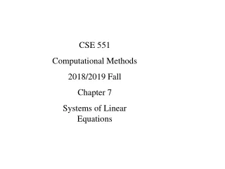
CSE 551 Computational Methods 2018/2019 Fall Chapter 7 Systems of Linear Equations
Outline Naive Gaussian Elimination Gaussian Elimination with Scaled Partial Pivoting Tridiagonal and Banded Systems
References • W. Cheney, D Kincaid, Numerical Mathematics and Computing, 6ed, • Chapter 7 • Chapter 8
Naive Gaussian Elimination A Larger Numerical Example Algorithm Pseudocode Testing the Pseudocode Residual and Error Vectors
Naive Gaussian Elimination • fundamental problems in many scientific and engineering applications is to • solve an algebraic linear system Ax = b • for the unknown vector x • the coefficient matrix A • and right-hand side vector b • known • arise – various applications; • approximating nonlinear equations by linear equations • or differential equations by algebraic equations • cornerstone of many numerical methods • the efficient and accurate solution of linear • systems • The system of linear algebraic equations Ax = b • may or may not have a solution • if it has a solution, it may or may not be unique.
Gaussian elimination – standard method for solving the linear system • When the system has no solution • other approaches, e.g., linear least squares • assume that: • the coefficient matrix A is n × n and • invertible (nonsingular) • pure mathematics - solution of Ax = b : x =A−1b • A−1:inverse matrix. • most applications - solve the system directly for the unknown vector x
many applications, daunting task: • to solve accurately extremely large systems - thousands or millions of unknowns • Some questions: • How to store such large systems in the computer? • Are computed answers correct? • What is the precision of the computed results? • Can the algorithm fail? • How long will it take to compute answers? • What is the asymptotic operation count of the algorithm? • Will the algorithm be unstable for certain systems? • Can instability be controlled by pivoting? (Permuting the order of the rows of the matrix is called pivoting.) • Which strategy of pivoting should be used? • Whether the matrix is ill-conditioned? • whether the answers are accurate?
Gaussian elimination transforms a linear system into an upper triangular form • easier to solve • process equivalent to finding the factorization • A = LU • L: unit lower triangular matrix • U: upper triangular matrix • This • useful solving many linear systems • the same coefficient matrix • different right-hand sides
When A - special structure: • symmetric, positive definite, triangular, banded, block, or sparse • Gaussian elimination with partial pivoting • modified or rewritten specifically for th system.
develop a good program for solving a system of n • linear equations in n unknowns: • In compact form:
A Larger Numerical Example • simplest form of Gaussian elimination - naive • not suitable for automatic computation • essential modifications • e.g., naive Gaussian elimination:
first step • elimination procedure: • certain multiples of the first equation • subtracted from the second, third, and fourth equations • eliminate x1 from these equations. • to create 0’s as coefficients for each x1 below the first • 12, 3, −6 stand • subtract 2 times the first equation from the second • multiplier: 12/6 . • subtract 12 times the first equation from the third • multiplier:3/6 • subtract −1 times the first equation from the fourth.
the first equation not altered pivot equation • Systems (2) and (3) are equivalent: • Any solution of (2) is also a solution of (3)
second step • ignore the first equation and the first column of coefficients • system of three equations with three unknowns same process repeated: • the top equation in the smaller system current pivot equation • subtracting 3 times the second equation from the third. • multiplier: −12/(-4) • subtract −1/2 times the second equation from the fourth
final step: • subtracting 2 times the third equation from the fourth: • system is in upper triangular form • equivalent to System (2)
completes first phase (forward elimination) • The second phase (back substitution) • solve System (5) for the unknowns starting at the • bottom • from the fourth equation: • Putting x4 = 1 in the third equation: • The solution:
Algorithm • write System (1) in matrix-vector form • ai j: n × n square array, or matrix • unknowns xi • right-hand side elements bi:n×1 arrays, or vectors • or
Operations between equations correspond to operations between rows in this notation • naive Gaussian elimination algorithm for the general system, • n equations and n unknowns • original data are overwritten
forward elimination phase • n − 1 principal steps • first step: first equation to produce n − 1 • zeros as coefficients for each x1 in all other equations i, i >1 • subtracting appropriate multiples of the first equation from the others • first equation - first pivot equation • a11 as the first pivot element
remaining equations (2 i n): • ← : replacement • content of the memory location allocated to ai jreplaced by ai j− (ai 1/a1 1)a1 j, and so on. • (ai1/a11) multipliers • new coefficient of x1 in the ith equation:0 • ai1 − (ai1/a11)a11 = 0.
not alter first equation • not alter coefficients x1 • a multiplier times 0 subtracted from 0 is still 0 • ignore the first row and the first column • repeat the process on the smaller system. • With the second equation - pivot equation: • compute for each remaining equation (3 i n)
prior to the kth step, the system: • a wedge of 0 coefficients created • first k equations processed - now fixed • kth equation - pivot equation • select multipliers - create 0’s coefficients xibelow the akkcoefficient.
compute for each remaining equation • (k + 1i n) • assume that all the divisors in this algorithm are nonzero
Pseudocode • pseudocode for forward elimination • coefficient array: (ai j ) • right-hand side of the system of equations: (bi ) • solution computed: (xi )
multiplier aik/akknot depend on j • moved outside the j loop • the new values in column k will be 0-theoretically, when j = k:
The location where the 0 created good place to store multiplie :
At the beginning of the back substitution phase, • the linear system: • the ai j’s and bi’s not original ones from System (6) • altered by the elimination process
The back substitution starts by solving the nth equation for xn: • using the (n − 1)th solve for xn−1: • continue upward, recovering each xi:
crucial computation: • a triply nested for-loop containing a replacement operation:
expect all quantities to be infected with roundoff error • Such a roundoff error • in ak jmultiplied by the factor (aik/akk) • large: pivot element |akk| small relative to |aik|. • conclude, tentatively, that • small pivot elements lead to • large multipliers and to worse roundoff errors.
Testing the Pseudocode • One way to test a procedure: • set up an artificial problem • solution is known beforehand • test problem - parameter • changed to vary the difficulty. • example: • Fixing n:
coefficients all equal to 1 • try to recover known coefficients • values of p(t) at integers t = 1+i for i = 1, 2, . . . , n • coefficients: x1, x2, . . . , xn: • used formula sum of a geometric series on the right-hand side: • linear system
Example • write a pseudocode for a specific test case that solves the system of Equation (8) for various values of n. • Solution: use Naive Gauss • calling program: n = 4, 5, 6, 7, 8, 9, 10 • for testing
run on a machine approximately seven decimal digits of accuracy • solution with complete precision until n reached 9, • then, the computed solution worthless • one component exhibited a relative error of 16,120%!
The coefficient matrix for this linear system • example of a well-known illconditioned • matrix the Vandermonde matrix • cannot be solved accurately - naive Gaussian elimination • amazing • the trouble happens so suddenly! n: 9 • roundoff error - computing xipropagated and magnified throughout the back substitution phase • most computed values for xiworthless • Insert intermediate print statements • to see what is going on hereRes
Residual and Error Vectors • linear system Ax = b - true solution x • and a computed solution • define: • relationship between the error vector and the residual vector:
using different computers solve the same linear system, Ax = b • algorithm and precision not known • two solutions xaand xbtotally different! • How determine which, if either, computed solution is correct?
check the solutions substituting them into the original system, • computing the residual vectors: ra= Axa− b and rb= Axb− b • computed solutions not exact • some roundoff errors • accept the solution with the smaller residual vector. • However, if we knew • the exact solution x, then we would just compare the computed solutions with the exact • solution, which is the same as computing the error vectors ea= x −xaand eb= x −xb • computed solution - smaller error vector • most assuredly be the better answer
exact solution not known • accept • the computed solution - smaller residual vector • may not be the best computed solution • original problem sensitive to roundoff errors • illconditioned. • the question: • whether a computed solution to a linear system is a good solution is extremely difficult
Gaussian Elimination with Scaled Partial Pivoting Naive Gaussian Elimination Can Fail Partial Pivoting and Complete Partial Pivoting Gaussian Elimination with Scaled Partial Pivoting A Larger Numerical Example Pseudocode Long Operation Count Numerical Stability Scaling
Naive Gaussian Elimination Can Fail • naive Gaussian elimination algorith - unsatisfactory: • the algorithm fails if a11 = 0. • If fails for some values of the data • untrustworthy - values near the failing values: • ε small number different from 0
naive algorithm works • after forward elimination: • back substitution: • ε−1 large - computer – fixed word length • small ε, (2 − ε−1),(1 − ε−1) computed as −ε−1
8-digit decimal machine with a 16-digit accumulator, when ε =10−9 • ε−1 = 109 • subtract -interpret the number: • ε−1−2computed: 0.09999 99998 00000 0 × 1010 rounded to 0.10000 000×1010 = ε−1
for values of ε sufficiently close to 0 • computer calculates x2:1 x1: 0 • correct solution: • relative error x1: 100%
naive Gaussian elimination algorithm works well on Systems (1) and (2) • if the equations are first permuted: x2 = 1, x1 = 2 - x2=1
second systems: • forward elimination and back substitution: • not to rearrange the equations • select a different pivot row • difficulty in (2): • not ε small but small relative to other coefficients in the same row