Read Once Branching Programs: a model of computation used in CAD.

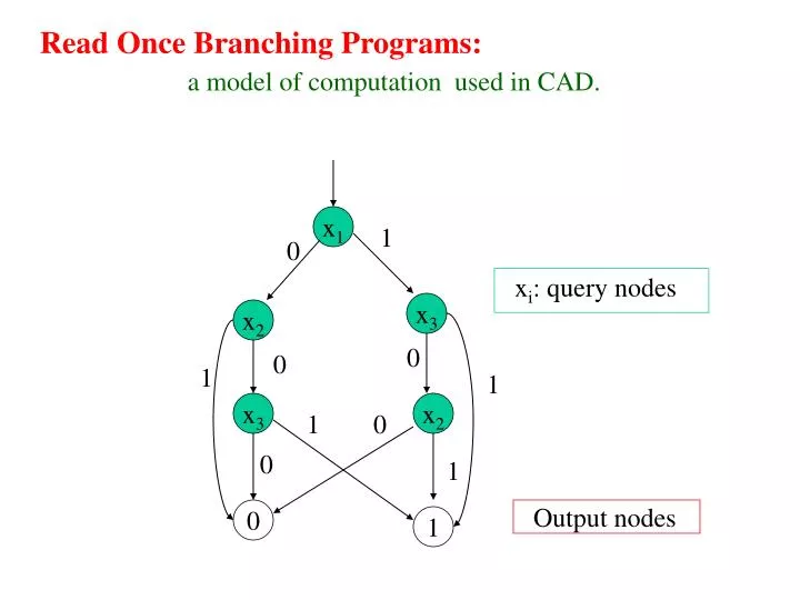
1. Read Once Branching Programs: a model of computation used in CAD. x1 1 0 xi: query nodes x3 x2 0 0 1 1 x3 x2 1 0 0 1 Output nodes 0 1

2. What is the ROBP for OR function with 4 variables?

3. Represent a BP with a polynomial: the polynomial for the output node 1. x p xp 1 (1-x)p 0 1 x1 (1- x1) 1 x1 0 x1 (1- x1) x3 x2 0 0 1 p1 …. pn 1 x2(1- x1) x3 x2 1 0 x p1+…+pn 0 1 0 1 0 1

4. Relationship between a ROBP B and the assigned polynomial p: For any Boolean assignment to B’s variables, all polynomials assigned to its nodes evaluate to 0 or 1. Polynomials evaluating to 1 are those on the computation path for that assignment. Hence B and p agree on Boolean input. Since B is read once, we may write p as a sum of product terms: y1y2….ym, where yi is xi , (1- xi) or 1 and each term correspond a path from the start node to the output node 1. If the path doesn’t contain xi thenyi =1 . Take each term of p with yi =1 and split it into xi and (1- xi). Doing this yields the same polynomial. Continue until all yi is either xi or (1- xi). The end result is an equivalent polynomial q that contains a product term for each assignment on which B evaluates to 1.

5. EQROBP= { <B1, B2> | B1 and B2 are equivalent ROBP }. Thm: EQROBPis in BPP. Proof: Suppose there are m variables in both ROBP’s. Transform both ROBP’s into polynomials as above. Let F be a field with at least 3m elements. D = “on input <B1, B2>: 1. Select randomly a1,…, am from F. 2. Evaluate the assigned polynomials p1 and p2 at ai’s. 3. If p1(a1,…, am ) = p2(a1,…, am ) accept; o/w reject.” If B1 and B2 are equivalent, then D always accepts, since they evaluate to 1 on exactly the same assignments. Else D rejects with a probability at least 2/3 by the following lemmas.

6. Lemma: For every d 0, a degree d polynomial p on a single variable x either has at most d roots, or it is a zero polynomial. Proof: By induction on d. It is obvious for d = 0, since degree-0 polynomial either has no root or is identical to zero.. Suppose it is true for d-1 and prove true for d. If p != 0 and of degree d with a root at a, then (x-a)|p and p/(x-a) is a non-zero polynomial of degree d-1 and has at most d-1 roots by induction hypothesis.

7. Lemma: Let F be a finite field with f elements and let p be a nonzero polynomial on the variables x1 through xm, where each variable has degree at most d. If a1 through am are selected randomly from F, thenPr[p(a1,…, am ) = 0]  md/f. Proof: By ind on m. For m=1, by the previous lemma, p has at most d roots, so the probability is at most d/f. Assume it is true for m-1 and prove for m. Represent p as p = p0+x1p1+…+x1d pd . If p(a1,…, am ) = 0, then either all pi evaluate to 0 or some p1 doesn’t evaluate to 0 and a1 is a root of the single variable poly obtained by evaluating p0 through pd on a2 through am.

8. p = p0+x1p1+…+x1d pd Since p is nonzero, there is a pj is nonzero. Pr[ all pi evaluate to 0 ] Pr[ pj evaluate to 0] (m-1)d/f, by induction hypothesis. If some pi doesn’t evaluate to 0, then on the assignment of a2 through am, p reduces to a nonzero single variable polynomial. The basis already shows that a1 is a root of such a poly with probability of at most d/f. Therefore, Pr[p(a1,…, am ) = 0]  (m-1)d/f +d/f = md/f.