Download
1 / 30
310 likes | 468 Views
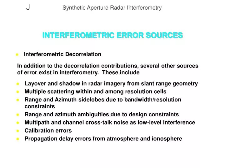
INTERFEROMETRIC ERROR SOURCES. Interferometric Decorrelation. In addition to the decorrelation contributions, several other sources of error exist in interferometry. These include. Layover and shadow in radar imagery from slant range geometry

E N D
INTERFEROMETRIC ERROR SOURCES • Interferometric Decorrelation In addition to the decorrelation contributions, several other sources of error exist in interferometry. These include • Layover and shadow in radar imagery from slant range geometry • Multiple scattering within and among resolution cells • Range and Azimuth sidelobes due to bandwidth/resolution constraints • Range and azimuth ambiguities due to design constraints • Multipath and channel cross-talk noise as low-level interference • Calibration errors • Propagation delay errors from atmosphere and ionosphere
LAYOVER AND SHADOW IN RADAR IMAGING Mapping of Earth’s surface into slant range distorts highly sloped areas RADAR IMAGE Slant Range TERRAIN Shadow Layover Ground Range
LAYOVER EFFECTS IN INTERFEROMETRY • As slopes increase and approach the look direction, the resolution element size normal to the look direction increases toward infinity. This has the following consequences: • Radar backscatter return becomes very bright, giving high interferometric correlation (high SNR) • Effective critical baseline decreases toward zero, with interferometric fringe rate approaching one cycle of phase per pixel No surface slope Surface slope
LAYOVER EFFECTS IN INTERFEROMETRY • The distortion of terrain into slant range coordinates has consequences for the inference of terrain height from interferometric phase • Widely spaced points on the sloping ground, well outside a particular ground resolution element, can contribute to the complex backscatter in a range resolution element, particularly when the slope exceeds the look angle, leading to incorrect heights. • The close proximity in slant range of widely space ground elements at very different heights leads to phase shears that confound phase unwrapping algorithms. Two scatterers with range Two scatterers with range
MULTIPLE SCATTERING EFFECTS • Layover illustration is also an example of multiple scattering effects that occur among resolution cells. In this case, the bridge return will dominate the water return. There will be multiple images of the bridge in the radar image at different ranges. Each range element in an interferogram will have its own interpretation of the height, depending on the scattering phase function of the bridge and water Similar effects occur within the volume of a resolution element in forming the coherent backscatter. The aggregate height is not necessarily the uniformly weighted average of the scatter heights Two scatterers with range Two scatterers with range
SHADOW EFFECTS IN INTERFEROMETRY • As slopes approach being parallel to the look direction, the resolution element size normal to the look direction decreases toward zero. This has the following consequences: • Radar backscatter return becomes very dim, giving low interferometric correlation (low SNR), adding difficulty to phase unwrapping • Effective critical baseline increases toward infinity, with interferometric fringe rate slowing down, easing phase unwrapping No surface slope Surface slope
LAYOVER AND SHADOW MITIGATION • For wide-swath interferometric systems that span a large range of incidence angles, the effects of layover and shadow can be mitigated through parallel track imaging: • Layover more likely in near swath where look angle is shallow • Shadow more likely in far swath where look angle is steep • By flying parallel tracks with partial swath overlap, near swath layover regions are likely to be intact in far swath of parallel track, and shadow regions in far swath are likely to be intact in near swath of a different parallel track • For narrow swath systems, orthogonal imaging geometries are probably best • Opposite side imaging (anti-parallel tracks) not optimal because near swath layover of one track corresponds to far swath shadow of anti-parallel track
EXAMPLE OF LAYOVER/SHADOW MITIGATION • Figure of Northridge Mosaic here.
RANGE SIDELOBES IN RADAR IMAGING • Range sidelobes arise in extended time-bandwidth implement-ations of linear FM pulsed systems. For a pulse of duration with chirp rate , observing a target located at temporal position , the impulse response is:
RANGE SIDELOBES IN INTERFEROMETRY • The interferometric phase associated with the main lobe of a resolution element contributes to the surrounding resolution elements weighted by the range impulse response • Phase noise contributed by range sidelobes usually modeled as additive noise term at the level NSR = ISLR. NSR is multiplied by expected signal level to compute noise power to add. • Range sidelobes actually contribute multiplicative noise: consider the case when the peak side lobe is brighter than the ambient backscatter Main lobe with interferometric phase side lobes with interferometric phase peak side lobe
AZIMUTH SIDELOBES IN RADAR IMAGING • Azimuth sidelobes arise in the naturally extended time-bandwidth environment of synthetic aperture systems. For a system with Fresnel zone , azimuth antenna length , observing a targe at azimuth location , the azimuth impulse response is: In interferometry, treatment of azimuth sidelobes is similar to range sidelobes
SIDELOBE MITIGATION STRATEGIES • In regions of high contrast, where sidelobes can lie above the ambient backscatter, or in regions that are are very dark and cannot tolerate a significant additional noise contribution, sidelobes must be reduced • Weighting of the matched filter function in range or azimuth compression can effectively reduce sidelobes in a controlled fashion • Cost of weighting is reduction in processing bandwidth, leading to reduction in resolution. • Design of an interferometer should consider bandwidth and weighting functions suited to the mapping problem of interest: e.g. urban mapping requires very fine resolution and very low sidelobes because the scenes are highly contrasted.
RANGE AMBIGUITIES IN INTERFEROMETRY • Range ambiguities arise in spaceborne systems primarily, because the radar must pulse faster than the round-trip light time for a single pulse event. • Because multiple pulses are in the air, it is possible for the tail end of energy from a preceding pulse or leading end of energy from a succeeding pulse to contribute to a pulse of interest. • Though multiplicative noise, range ambiguities are modeled as additive thermal noise at a level NSR = total power integrated in ambiguous pulses within the swath. This noise ratio multiplied by the expected mean signal power sets the additive noise level. This roughly determines the interferometric phase noise contributed to the system. • Through adjustment of the pulse width and the pulse repetition frequency, it is possible to control range ambiguities.
ILLUSTRATION OF RANGE AMBIGUITIES • Range ambiguity figure here
AZIMUTH AMBIGUITIES IN RADAR IMAGING • Azimuth ambiguities arise in radar imaging because the pulse repetition frequency is insufficient to satisfy the Nyquist criterion for adequate sampling of the Doppler spectrum. • Spaceborne systems are typically designed for low PRF, near the 3dB spectral width, to reduce data rate. As a result, energy in the tails of the azimuth spectrum aliases. • Azimuth ambiguities are again multiplicative, but are modeled in the usual additive way. Limiting the processing bandwidth to a fraction of the PRF reduces ambiguity level f PRF
AMBIGUITY MITIGATION STRATEGY • Range and azimuth ambiguities contribute to the random phase noise in interferometry multiplicatively. • Both range and azimuth ambiguities rising above the ambient backscatter significantly corrupt the interferometric phase. • To reduce azimuth ambiguities, PRF should be increased to properly sample azimuth spectrum. • To reduce range ambiguities, PRF should be decreased (in general) to separate pulses in time as much as possible. • Trade-off must consider the required azimuth resolution, desired look angles, swath width, and noise level.
INTERFEROMETRIC RADAR SCHEMATIC In addition to baseline and position, time and phase delays in the radar require calibration.
CALIBRATION PARAMETER EQUATIONS The phase at the receiver outputs is given by Baseband frequency: Receiver time delay: Transmitter phase delay:
CALIBRATION PARAMETER EQUATIONS II The phase difference between the channels is Channel phase constant: If total time and phase delay differences can be measured, then range difference proportional to topography (final term in equation) can be known. Note: this term is also dependent on baseline know- ledge accuracy.
CALIBRATION STRATEGIES • To determine the channel time and phase delays, assume that the interferometer is stable over time and baseline is known. • Total time delay (range) can be determined by comparing location of known target to inferred location • Differential time delay can be determined by scene matching over a flat surface • Differential phase delay can be determined by inserting a calibration tone near the receiving antennas
CALIBRATION STRATEGIES II • It is also possible to calibrate the radar interferometer through simultaneous least squares adjustment, utilizing the sensitivity equations described earlier and reference data, such as a DEM • Requires radar receiver time and phase stability over all time, which is difficult to achieve • Requires baseline stability over all time • Least squares adjustment and calibration tone is generally needed • One solution to potentially remove receiver delays without calibration tone: operate the interferometer in “ping-pong” mode. • By using a single transmitter and receiver, differential time and phase delays are zero. • Cost: double pulse repetition frequency for the one receiver required to properly sample azimuth spectrum.
CHANNEL ISOLATION IN RADAR INTERFEROMETRY • In some single-pass dual-aperture systems, energy can leak between receiver channels • Standard mode: radiation from other antenna or platform scatterers entering the antenna (multipath) • Ping-pong mode: switch between receiving antennas has some leakage, and multipath • Switch leakage and multipath from other antenna appear in interferometric phase signature as phase modulation at the interferometric fringe frequency. • Multipath from other platform scattering sources appears as phase modulation at a frequency proportional to the scatterer-antenna separation. • Repeat-pass single-aperture systems do not suffer from channel isolation problems.
SWITCH ISOLATION with leakage In ping-pong operation, switch alternates antenna setting for transmit/receive.
SWITCH ISOLATION II First term of Expression First two terms All three terms
ANTENNA MULTIPATH IN INTERFEROMETRY Baseline B is constant. Multipath off antennas has same effect as switch leakage.
PLATFORM MULTIPATH Multipath cross terms depend on “baseline” from platform scatterer
ATMOSPHERIC PROPAGATION EFFECTS IN RADAR INTERFEROMETRY • Due to turbulent mixing in the troposphere, particularly in the wet layers, the refractive index along the radar ray path varies within the scene. • Wet tropospheric variations of refractivity are typically an order of magnitude smaller than the dry troposphere total path refractivity because the wet troposphere is concentrated in a layer near the earth’s surface. • For single-pass two-aperture systems, the difference in path delay variations cancels to first order because the ray path sensed is nearly identical. The total path delay does affect the absolute range, as seen previously, but not significantly the differential range or phase. • For repeat-pass single-aperture systems, the difference in path delay is a substantial limiting factor.
IONOSPHERIC PROPAGATION EFFECTS IN RADAR INTERFEROMETRY • Due to turbulent mixing in the ionosphere, and diurnal variations of earth’s response to the solar wind, the refractive index along the radar ray path varies within the scene. • For airborne systems, the ionosphere is not a concern. • For spaceborne platforms, the scale size of ionospheric anomalies is large in the radar scene because the ionosphere is relatively close to the sensor. • For single-pass two-aperture systems, the difference in path delay variations cancels to first order because the ray path sensed is nearly identical. • For repeat-pass single-aperture systems, the difference in path delay is a substantial limiting factor.