Download

1 / 72
720 likes | 841 Views
20. 18. 16. 14. 12. 10. 8. 6. X1. 4. 2. 2. 0. 0. An Animated Instructional Module. for Teaching Production Economics. with the Aid of. Three-Dimensional Graphics. David L. Debertin. University of Kentucky. Y. 250. 167. 83. 0. 20. 18. 16. 14. 12. 10. 8. X2. 6. 4.

E N D
20 18 16 14 12 10 8 6 X1 4 2 2 0 0 An Animated Instructional Module for Teaching Production Economics with the Aid of Three-Dimensional Graphics David L. Debertin University of Kentucky Y 250 167 83 0 20 18 16 14 12 10 8 X2 6 4
This instructional module is based on the polynomial production function 2 3 2 y = x + x - 0.05 x + x + x 1 2 1 1 2 3 - 0.05 x + 0.4 x x . 2 1 2 This production function was chosen for a number of reasons.
1. It possesses a region of increasing marginal returns, a region of diminishing marginal returns and a region of negative marginal returns to the variable inputs x and x . 2 1 2 dy = 1 + 2 x - 0.15 x + 0.4 x . 1 1 2 dx 1 2 dy = 1 + 2 x - 0.15 x + 0.4 x . 2 2 1 dx 2
2. Since the function has a finite maximum, there are "ring" isoquants, centered at the maximum output level. At the maximum output level, dy and dy are both zero. dx dx 1 2 Maximum output is 237.21 units corresponding to x = x = 16.41 units 1 2
3. There is a global point of profit maximization. This point occurs at an output level less than the global point of profit maximization. For example, if the price of the product (y) is $1.00 per unit, the price of x is $3.00 1 per unit, and the price of x is $1.50 per unit, 2 then profit is maximum at x =15.21 and x = 15.71 1 2 units. Total Revenue is $234.85; Total Cost for x and x is $69.20; 1 2 Profit is Total Revenue - Total Cost = $165.20
In the following sequence, the production surface for the polynomial is sliced horizontally at various levels. The isoquant at each output level appears in red. Note that isoquants at low output levels are concave to the origin, but as the output level increases, the isoquants become convex to the origin. You are looking at the 3-D surface from the origin. x is at your right; x at your left. 2 1 Output (y) is measured on the vertical axis.
Y 250 167 83 0 20 20 18 18 16 16 14 14 12 12 10 10 8 8 6 X1 X2 6 4 4 2 2 0 0
Y 250 167 83 0 20 20 18 18 16 16 14 14 12 12 10 10 8 8 6 X1 X2 6 4 4 2 2 0 0
Y 250 167 83 0 20 20 18 18 16 16 14 14 12 12 10 10 8 8 6 X1 X2 6 4 4 2 2 0 0
Y 250 167 83 0 20 20 18 18 16 16 14 14 12 12 10 10 8 8 6 X1 X2 6 4 4 2 2 0 0
Y 250 167 83 0 20 20 18 18 16 16 14 14 12 12 10 10 8 8 6 X1 X2 6 4 4 2 2 0 0
Y 250 167 83 0 20 20 18 18 16 16 14 14 12 12 10 10 8 8 6 X1 X2 6 4 4 2 2 0 0
Y 250 167 83 0 20 20 18 18 16 16 14 14 12 12 10 10 8 8 6 X1 X2 6 4 4 2 2 0 0
Y 250 167 83 0 20 20 18 18 16 16 14 14 12 12 10 10 8 8 6 X1 X2 6 4 4 2 2 0 0
Y Y 250 250 167 167 83 83 0 0 20 20 20 20 18 18 18 18 16 16 16 16 14 14 14 14 12 12 12 12 10 10 10 10 8 8 8 8 6 6 X1 X1 X2 X2 6 6 4 4 4 4 2 2 2 2 0 0 0 0
Y 250 167 83 0 20 20 18 18 16 16 14 14 12 12 10 10 8 8 6 X1 X2 6 4 4 2 2 0 0
Y Y 250 250 167 167 83 83 0 0 20 20 20 20 18 18 18 18 16 16 16 16 14 14 14 14 12 12 12 12 10 10 10 10 8 8 8 8 6 6 X1 X1 X2 X2 6 6 4 4 4 4 2 2 2 2 0 0 0 0
Y 250 167 83 0 20 20 18 18 16 16 14 14 12 12 10 10 8 8 6 X1 X2 6 4 4 2 2 0 0
Y Y 250 250 167 167 83 83 0 0 20 20 20 20 18 18 18 18 16 16 16 16 14 14 14 14 12 12 12 12 10 10 10 10 8 8 8 8 6 6 X1 X1 X2 X2 6 6 4 4 4 4 2 2 2 2 0 0 0 0
Y 250 167 83 0 20 20 18 18 16 16 14 14 12 12 10 10 8 8 6 X1 X2 6 4 4 2 2 0 0
Y Y 250 250 167 167 83 83 0 0 20 20 20 20 18 18 18 18 16 16 16 16 14 14 14 14 12 12 12 12 10 10 10 10 8 8 8 8 6 6 X1 X1 X2 X2 6 6 4 4 4 4 2 2 2 2 0 0 0 0
Y 250 167 83 0 20 20 18 18 16 16 14 14 12 12 10 10 8 8 6 X1 X2 6 4 4 2 2 0 0
Y Y 250 250 167 167 83 83 0 0 20 20 20 20 18 18 18 18 16 16 16 16 14 14 14 14 12 12 12 12 10 10 10 10 8 8 8 8 6 6 X1 X1 X2 X2 6 6 4 4 4 4 2 2 2 2 0 0 0 0
Y 250 167 83 0 20 20 18 18 16 16 14 14 12 12 10 10 8 8 6 X1 X2 6 4 4 2 2 0 0
Y Y 250 250 167 167 83 83 0 0 20 20 20 20 18 18 18 18 16 16 16 16 14 14 14 14 12 12 12 12 10 10 10 10 8 8 8 8 6 6 X1 X1 X2 X2 6 6 4 4 4 4 2 2 2 2 0 0 0 0
In the following sequence, isoquants representing various output levels appear in different colors and the output level represented by each isoquant corresponds with the key at the bottom of the chart.
The budget constraint is represented by red lines of constant slope P1/P2 where P1 is the price of input x , and P2 is the price of input 1 x . 2 Increases in the amount of money available for the purchase of inputs shift the budget constraint outward. Each budget constraint is tangent (just touches) an isoquant. These points, here marked by blue circles, are where P1/P2 = the Marginal Rate of Substitution of x for x . 1 2
Valid constrained output maximization points are only those on isoquants that are convex to the origin of the graph. Points on concave isoquants are constrained output minimization points, and are marked with a yellow X. The expansion path connects valid points of constrained output maximization, and is shown in green.
Ridge line 1 connects all points of zero slope on the isoquants. Ridge line 2 connects all points of infinite slope on the isoquants. Ridge lines, shown here in blue-green intersect at the global point of output maximization. This occurs at x = x = 16.41 and y = 237.21. 1 2
Pseudo Scale Line 1 connects profit maximization points for x holding x constant. 1 2 Each point on Pseudo Scale Line 1 is defined by MPP x = P1/Py, where P1 is the price of x and 1 1 Py is the output price. Pseudo Scale Line 2 connects profit maximization points for x holding x constant. 2 1 Each point on Pseudo Scale Line 2 is defined by MPP x = P2/Py, where P2 is the price of x and 2 2 Py is the output price. Pseudo Scale Lines, shown here in orange, Converge at the point of global profit maximization.
What happens to Pseudo Scale Lines and the position of the Expansion Path when one of the input prices changes is also shown. First, P2 (the price of x ) is increased. 2 Pseudo Scale Line 2 moves in from Ridge Line 2, and the Expansion Path now favors the use of the now relatively cheaper input x . 1 Then P2 (the price of x ) is decreased. 2 Pseudo Scale Line 2 moves toward Ridge Line 2, and the Expansion Path now favors the use of the now relatively cheaper input x . 2 Pseudo scale line 1 has not moved in either case as the price of x has not changed. 1
X2 20 18 16 14 12 10 8 6 4 2 0 X1 0 2 4 6 8 10 12 14 16 18 20 Y 0 24 47 71 95 119 142 166 190 213 237
X2 20 18 16 14 12 10 8 6 4 2 P1 P2 0 X1 0 2 4 6 8 10 12 14 16 18 20 Y 0 24 47 71 95 119 142 166 190 213 237
X2 20 18 16 14 12 10 8 6 X X 4 X 2 P1 P2 0 X1 0 2 4 6 8 10 12 14 16 18 20 Y 0 24 47 71 95 119 142 166 190 213 237
X2 20 Global 18 Output Maximum 16 Expansion 14 Path 12 10 8 6 X X 4 X 2 P1 P2 0 X1 0 2 4 6 8 10 12 14 16 18 20 Y 0 24 47 71 95 119 142 166 190 213 237
X2 20 Global 18 Output Maximum 16 Expansion 14 Path 12 10 8 6 X X 4 X 2 P1 P2 0 X1 0 2 4 6 8 10 12 14 16 18 20 Y 0 24 47 71 95 119 142 166 190 213 237
X2 20 Global 18 Output Maximum Ridge 16 Line 2 Expansion 14 Path 12 10 8 6 X X 4 X 2 P1 Ridge Line P2 1 0 X1 0 2 4 6 8 10 12 14 16 18 20 Y 0 24 47 71 95 119 142 166 190 213 237
X2 20 Global 18 Output Maximum Ridge 16 Line 2 Expansion 14 Path 12 MPPx2= Px2/Py 10 8 6 X X 4 MPPx1 = X Px1/Py 2 P1 Ridge Line P2 1 0 X1 0 2 4 6 8 10 12 14 16 18 20 Y 0 24 47 71 95 119 142 166 190 213 237
X2 20 Global 18 Output Maximum Ridge 16 Global Line Profit 2 Maximum Expansion 14 Pseudo Path Scale Line 2 12 MPPx2= Px2/Py 10 8 6 X X Pseudo 4 Scale Line 1 MPPx1 = X Px1/Py 2 P1 Ridge Line P2 1 0 X1 0 2 4 6 8 10 12 14 16 18 20 Y 0 24 47 71 95 119 142 166 190 213 237
X2 20 Global 18 Output Maximum Ridge 16 Line 2 Expansion 14 Global Path Profit Maximum 12 Pseudo Scale Line 2 MPPx2= 10 Px2/Py 8 X 6 Pseudo X 4 Scale Line 1 MPPx1 = Px1/Py P1 2 Ridge P2 Line 1 0 X1 0 2 4 6 8 10 12 14 16 18 20 Y 0 24 47 71 95 119 142 166 190 213 237
X2 20 Global 18 Global Output Profit Maximum Maximum Ridge 16 Line 2 Line 2 Scale Pseudo 14 MPPx2= X Px2/Py 12 Expansion Path 10 8 6 Pseudo 4 Scale Line 1 MPPx1 = Px1/Py P1 2 Ridge P2 Line 1 X X 0 X1 0 2 4 6 8 10 12 14 16 18 20 Y 0 24 47 71 95 119 142 166 190 213 237
In the following sequence, vertical slices of the production surface are made. The slice is at the budget constraint angle relative to the origin of the graph. Each slice represents a different level of the budget constraint. The locus ABC represents the function being maximized or minimized in the constrained optimization problem. If B is lower than A or C, then the function is being minimized. If B is higher than A or C, then the function is being maximized.
Y 250 167 83 0 20 20 18 18 16 16 14 14 12 12 10 10 8 8 6 X1 X2 6 4 4 2 2 0 0
Y 250 167 83 0 20 20 18 18 16 16 14 14 12 A C 12 B 10 10 8 8 6 X1 X2 6 4 4 2 2 0 0
Y 250 167 83 0 20 20 18 A C 18 16 B 16 14 14 12 12 10 10 8 8 6 X1 X2 6 4 4 2 2 0 0
Y 250 167 83 A C B 0 20 20 18 18 16 16 14 14 12 12 10 10 8 8 6 X1 X2 6 4 4 2 2 0 0
Y 250 167 83 B C A 0 20 20 18 18 16 16 14 14 12 12 10 10 8 8 6 X1 X2 6 4 4 2 2 0 0
Y 250 167 B 83 A C 0 20 20 18 18 16 16 14 14 12 12 10 10 8 8 6 X1 X2 6 4 4 2 2 0 0
Y 250 B 167 83 A C 0 20 20 18 18 16 16 14 14 12 12 10 10 8 8 6 X1 X2 6 4 4 2 2 0 0
Y 250 B 167 83 A C 0 20 20 18 18 16 16 14 14 12 12 10 10 8 8 6 X1 X2 6 4 4 2 2 0 0