Download
1 / 46
460 likes | 562 Views
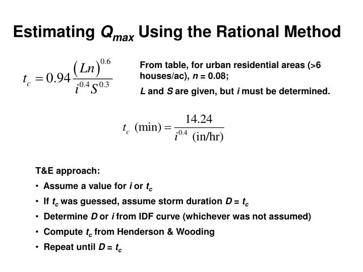
Estimating Q max Using the Rational Method. From table, for urban residential areas (>6 houses/ac), n = 0.08; L and S are given, but i must be determined. T&E approach: Assume a value for i or t c If t c was guessed, assume storm duration D = t c

E N D
Estimating Qmax Using the Rational Method From table, for urban residential areas (>6 houses/ac), n = 0.08; L and S are given, but i must be determined. • T&E approach: • Assume a value for i or tc • If tc was guessed, assume storm duration D = tc • Determine D or i from IDF curve (whichever was not assumed) • Compute tc from Henderson & Wooding • Repeat until D = tc
Estimating Qmax Using the Rational Method Guess tc= 5 min; For D = 5 min, i for 10-yr storm is 2.20 in/hr Guess tc= 10 min; For D = 10 min, i for 10-yr storm is 1.75 in/hr Guess tc= 12 min; For D = 12 min, i for 10-yr storm is 1.60 in/hr
Estimating Qmax Using the Rational Method From Table of runoff coefficients, C for dense residential area with rolling terrain is 0.75 (for Q in cfs, i in in/hr and A in ac). Using tc= D = 12 min, i = 1.60 in/hr:
Design For Runoff Conveyance • SCS method estimates tc in three categories • Shallow concentrated flow (e.g., in gullies) • Sheet flow over the land surface • Channel flow, in clearly-defined channels Shallow Concentrated Flow t = flow time (hr) n = Manning’s coef. for effective roughness for overland flow L = flow length (m or ft) P2 = 2-yr, 24-hr rainfall (cm or in) S = slope C = 0.029 (metric), 0.007 (US)
Design For Runoff Conveyance Sheet Flow and Channel Flow Both modeled using t = L/V, with V computed from Manning Eqn. For sheet flow, values of Rh and n assumed for two surface types: Paved: Rh = 0.2 ft, n = 0.025 Unpaved: Rh = 0.4 ft, n = 0.050 Yielding: with w = 16.1 ft/s (4.91 m/s) for paved and 20.3 ft/s (6.19 m/s) for unpaved
Design For Runoff Conveyance • Estimating Qmax using the SCS (NRCS) Method • Multi-step empirical equations leading to estimate of Qmax • Choose total precipitation, P (not Tr), for design storm • Determine CN for area and conditions of interest; use P and CN to estimate Ia / P from Table 2-10
Design For Runoff Conveyance • Estimating Qmax using the SCS (NRCS) Method • Multi-step empirical equations leading to estimate of Qmax • Use estimated Ia / P and SCS Storm Type (IA, I, II, or III) to estimate coefficients C0, C1, C2 from Table 2-9 • Insert coefficients and tc into equations on p.64 to estimate Qmax qu is “unit peak flow rate” in cfs per mi2 of watershed area per inch of precipitation (csm/in)
Design For Runoff Conveyance • Qmax from the SCS (NRCS) Method
Runoff Hydrographs and Design for Runoff Capture A Model Runoff Hydrograph Observed runoff is the composite result of continuously changing excess precipitation intensity (or, in this case, three idealized periods of constant intensity).
Design For Runoff Capture • The Unit Hydrograph • A hydrograph showing (precipitation and) runoff vs time for a storm producing a unit amount (1 cm or 1 in) of runoff • Assumes uniform intensity of runoff-producing precipitation, so duration of precipitation equals unit amount of runoff (1 cm or 1 in) divided by uniform intensity; i.e., for D of 0.25 hr, i is 4 in/hr. (Note: this is just for a conceptual storm; the real storm need not be that intense for the method to be used.) • Different unit hydrographs apply for different (i, D) pairs
Design For Runoff Capture • Actual runoff hydrographs for the watershed are assumed to be linear additions of unit hydrographs, weighted by intensity and staggered in time Composite hydrograph is modeled as sum of three contributing hydrographs, all with same pattern, but offset in their start times and with different magnitudes. Each component’s contribution is the unit hydrograph * actual intensity of excess precipitation divided by intensity that would produce unit runoff.
Design For Runoff Capture • Ideally, unit hydrographs are developed for individual watersheds, but SCS has proposed a universal approach for estimating hydrographs if no other data are available. The approach specifies a universal pattern for hydrograph shape as fcn of time and magnitude of peak Q.
Using the SCS Dimensionless Unit Hydrograph Qup is peak ‘unit’ runoff, in ft3/s per inch of total runoff; A in mi2, tp in hr; for units of m3/s per cm, km2, and hr, coefficient is 2.08 To develop unit hydrograph for desired duration, multiply values on x and y axes of standard, dimensionless SCS hydrograph by tp and Qup, respectively. (Applicable for D tc/6.)
A Synthetic Runoff Hydrograph Using the SCS Universal Unit Hydrograph Example. An urban watershed has a projected area of 0.63 mi2 and a time of concentration of 1.25 hr. Develop the 10-min unit hydrograph for the watershed, using the SCS universal unit hydrograph. Estimate lag time: Estimate time to peak flow: Estimate peak unit flow: Multiply x and y values of unit hydrograph by tp and Qup to develop graph
A Synthetic Runoff Hydrograph Using the SCS Universal Unit Hydrograph
Example. Predict the runoff hydrograph from the watershed described in the preceding example, for a storm that lasts one hour, with average, sequential 10-min excess precipitation intensities of 0.4, 0.8, 0.7, 0.3, 0.2, and 0.2 in/hr. Each 10-min portion of the storm contributes in proportion to its intensity.
Example. Predict the runoff hydrograph from the watershed described in the preceding example, for a storm that lasts one hour, with average, sequential 10-min excess precipitation intensities of 0.4, 0.8, 0.7, 0.3, 0.2, and 0.2 in/hr. Cumulative hydrograph is summation of contributing portions.
Detention Ponds: Storage Typical Storage vs. Stage relationship, from geometry
Detention Ponds: Outlets Develop Discharge vs. Stage relationship from standard equations for outlet structures
Spillway Detention Ponds:Stage vs Discharge for Parallel Outlets
Detention Ponds:Stage vs Discharge for Series Outlets In parallel, so additive In series, so lower Q controls
Modeling Detention Pond Dynamics Mass Balance on Water in Pond: Identical to Storage Analysis for Water Supply Or, in Finite Difference Form:
Modeling Detention Pond Dynamics At initial condition (n = 0), S0, I0, and Q0 are known. Choose a reasonable Dt, and identify I1 from runoff hydrograph, leaving two unknowns (S1 and Q1). Also know Q vs S relationship from Q vs h and S vs h. So: Guess S1, determine Q1 from Q vs S, and test whether those values satisfy the mass balance; if not, make a better guess and repeat.
Modeling Detention Pond Dynamics Akam suggested an approach that eliminates iteration: Re-write mass balance to put all knowns on left, unknowns on right: • Determine Q vs. S relationship • Pick Dt and, using Q vs. S relationship, plot (2S/Dt +Q) vs Q. • For n = 0, compute LHS of above eqn. This value equals RHS, which is 2S1/Dt + Q1. • Use the plot prepared in Step 2 to find value of Q1 that corresponds to the 2S1/Dt + Q1 found in Step 3. • Use the Q vs S relationship with Q1 (from Step 4) to find S1. • Now, all parameter values at n = 1 are known, and the process can be repeated to find the conditions at n = 2, etc.
Example. The storage (from geometry) and discharge (from outlet structure equations) as a function of stage for a storage pond are as shown in the following (incomplete) table and graphs. The runoff hyetograph for a design storm is also shown. Predict the discharge hydrograph from the pond, if it is empty at t=0. How much will the peak flow be attenuated?
Compute and Plot the “Storage Indication” Curve ** For Dt chosen to be 10 min
Determine Q vs. S relationship • Pick Dt (10 min, in this case) and, using Q vs. S relationship, plot (2S/Dt +Q) vs Q. • For n = 0, compute LHS of above eqn. I0=0, I1=20 ft3/s, S0=0, Q0=0 LHS1 =20 ft3/s. • Use the plot prepared in Step 2 to find Q1. RHS = LHS = 20 ft3/s; Q1≈0.5 ft3/s; h1≈0.1 ft. • Use the Q vs S relationship with Q1 (from Step 4) to find S1≈5500 ft3. • Now, all parameter values at n = 1 are known, and the process can be repeated to find the conditions at n = 2, etc.
Pond Inflow and Outflow Peak decreases from 252 to 184 ft3/s
Detention Pond Design • Design is based on mass balance on water, but exact steps are site-specific and difficult to generalize. Discharge hydrograph and discharge peak both depend on runoff hydrograph (which depends on IDF relationships) and on Stage-Storage-Discharge relationships. • Assuming design objective is to not exceed pre-development peak runoff, it is not clear initially which IDF point is critical for design. Can use synthetic hydrology to explore hypothetical storms long into the future to identify critical storm. • Stage-Storage-Discharge relationships can be controlled in many ways (shape of basin, number and type of outlet structures), each of which has different effects on the discharge hydrograph.
Detention Pond Design SCS has proposed a guideline for a preliminary choice of storage volume (Vs), based on a generic graph (on next slide). Still, many system parameters must be chosen arbitrarily, and sensitivity of discharge characteristics and cost to those parameters tested. Interpretation: If you want to have the peak outflow rate equal the fraction of the inflow rate given by the value on the x axis, you need to capture and store the fraction of total runoff shown on the y axis. If you do that, when the maximum volume of water is stored, the outflow rate will be the design peak rate; that rate can then be used to size the outlet structure, as shown in the following example.
Example. A detention basin is to be built to serve a 75-acre watershed with Type II rainfall. A preliminary stage-storage relationship is shown below. The outlet will be a weir with kw=0.40. The design objective is to reduce the peak flowfrom a 25-yr storm with 3.4 inches of runoff from 360 ft3/s to 180 ft3/s. Choose the storage volume using the SCS method, and determine the required weir length, if the crest is at elevation 100 ft. (Note: water might be present at Elev<100 ft, but since the weir crest is at 100 ft, the water below that elevation never drains, and that volume is not available storage.)
Solution. We are given the peak inflow (Ip, 360 ft3/s) and peak allowable outflow (Qp, 180 ft3/s), so Qp/Ip=0.50. From the graph, to achieve this reduction in peak flow from a Type II storm, Vs/Vr should be 0.28. So: The stage-storage relationship indicates that when Vs is 5.94 ac-ft, the stage is 105.7 ft, and the head above the crest is 5.7 ft.When the pond is at this stage, it must release the design peak flow. Rearranging the weir equation, we find the required length:
El 100 ft Example. It is desired to use the detention basin from the preceding example to also limit the 2-yr discharge rate to 50 ft3/s. The runoff and peak runoff rate from the 2-yr storm are 1.5 inches and 91 ft3/s, respectively. Design a two-stage weir, with the crest of the lower weir at elevation 100 ft, to achieve the design goal.
El 103.6 ft El 100 ft 2.3 ft Solution. Consider the 2-yr storm first. Ip is 91 ft3/s, and Qp is 50 ft3/s, so Qp/Ip=0.55. From the graph, Vs/Vris therefore 0.26. So: When Vs is 2.4 ac-ft, the stage is 103.6 ft. Since the crest is at 100 ft, the head above the crest is 3.6 ft, and:
Now design the upper weir. The maximum stage for the 25-yr storm remains the same as in the previous example – 105.7 ft. At this condition, flow over the lower weir is: Flow over the upper weir must therefore be (180 100)ft3/s. The head above the crest is (105.7 103.6), or 2.1 ft, so L is:
4.1 ft 4.1 ft El 105.7 ft El 103.6 ft El 100 ft 2.3 ft 4.1 ft El 105.7 ft El 100 ft Comparison of Weir Designs