Download
1 / 63
670 likes | 976 Views
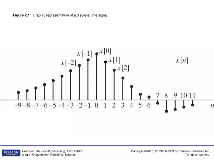
Figure 2.1 Graphic representation of a discrete-time signal. Figure 2.2 (a) Segment of a continuous-time speech signal x a (t ) . (b) Sequence of samples x [ n ] = x a (nT ) obtained from the signal in part (a) with T = 125 µ s.

E N D
Figure 2.1 Graphic representation of a discrete-time signal.
Figure 2.2 (a) Segment of a continuous-time speech signal xa(t ). (b) Sequence of samples x[n] = xa(nT ) obtained from the signal in part (a) with T = 125 µs.
Figure 2.3 Some basic sequences.The sequences shown play importantroles in the analysis and representationof discrete-time signals and systems.
Figure 2.4 Example of a sequence to be represented as a sum of scaled, delayed impulses.
Figure 2.5 cos ω0n for several different values of ω0. As ω0 increases from zero toward π (parts a-d), the sequence oscillates more rapidly. As ω0 increases from π to 2π (parts d-a), the oscillations become slower.
Figure 2.6 Representation of a discrete-time system, i.e., a transformation that maps an input sequence x[n] into a unique output sequence y[n].
Figure 2.7 Sequence values involved in computing a moving average with M1 = 0 and M2 = 5.
Figure 2.8 Representation of the output of an LTI system as the superposition of responses to individual samples of the input.
Figure 2.9 Forming the sequence h[n − k]. (a) The sequence h[k] as a function of k. (b) The sequence h[−k] as a function of k. (c) The sequence h[n − k] = h[ − (k − n)] as a function of k for n = 4.
Figure 2.10 Sequence involved in computing a discrete convolution. (a)–(c) The sequences x[k] and h[n− k] as a function of k for different values of n. (Only nonzero samples are shown.) (d) Corresponding output sequence as a function of n.
Figure 2.11 (a) Parallel combination of LTI systems. (b) An equivalent system.
Figure 2.12 (a) Cascade combination of two LTI systems. (b) Equivalent cascade. (c) Single equivalent system.
Figure 2.13 Equivalent systems found by using the commutative property of convolution.
Figure 2.14 An accumulator in cascade with a backward difference. Since the backward difference is the inverse system for the accumulator, the cascade combination is equivalent to the identity system.
Figure 2.15 Block diagram of a recursive difference equation representing an accumulator.
Figure 2.16 Block diagram of the recursive form of a moving-average system.
Figure 2.17 Ideal lowpass filter showing (a) periodicity of the frequency response and (b) one period of the periodic frequency response.
Figure 2.18 Ideal frequency-selective filters. (a) Highpass filter. (b) Bandstop filter. (c) Bandpass filter. In each case, the frequency response is periodic with period 2π. Only one period is shown.
Figure 2.19 (a) Magnitude and (b) phase of the frequency response of the moving-average system for the case M1 = 0 and M2 = 4.
Figure 2.20 Illustration of a real part of suddenly applied complex exponential input with (a) FIR and (b) IIR.
Figure 2.21 Convergence of the Fourier transform. The oscillatory behavior at ω = ωcis often called the Gibbs phenomenon.
Figure 2.22 Frequency response for a system with impulse response h[n] = anu[n]. (a) Real part. a > 0; a = 0.75 (solid curve) and a = 0.5 (dashed curve). (b) Imaginary part. (c) Magnitude. a > 0; a = 0.75 (solid curve) and a = 0.5 (dashed curve). (d) Phase.