Download
1 / 98
1.01k likes | 1.15k Views
Winds of Change:. Evolution of the El Ni ño Southern Oscillation (ENSO) from the Last Ice Age to Today. Andy Bush Dept. of Earth & Atmospheric Sciences University of Alberta. Winds of Change:. Evolution of the El Ni ño Southern Oscillation

E N D
Winds of Change: Evolution of the El Niño Southern Oscillation (ENSO) from the Last Ice Age to Today Andy Bush Dept. of Earth & Atmospheric Sciences University of Alberta
Winds of Change: Evolution of the El Niño Southern Oscillation (ENSO) from the Last Ice Age to Today Andy Bush Dept. of Earth & Atmospheric Sciences University of Alberta A.B.G. Bush, 2006, Journal of Climate, in press.
Winds of Change: Evolution of the El Niño Southern Oscillation (ENSO) from the Last Ice Age to Today Andy Bush Dept. of Earth & Atmospheric Sciences University of Alberta A.B.George Bush, 2006, Journal of Climate, in press.
Winds of Change: Evolution of the El Niño Southern Oscillation (ENSO) from the Last Ice Age to Today Andy Bush Dept. of Earth & Atmospheric Sciences University of Alberta A.B.George Bush, 2006, Journal of Climate, in press. andrew.bush@ualberta.ca
Motivation: To understand the climatological factors that determine the period and intensity of interannual variability (ENSO).
Motivation: To understand the climatological factors that determine the period and intensity of interannual variability (ENSO). Past climates provide altered mean states within which interannual variability exists.
Some human impacts of ENSO: 1) Impact on disease spread (malaria and dengue) 2) Food production
Observed Composite Temperature Anomalies El Niño La Niña
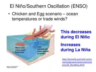
Existing numerical models for ENSO prediction are • anomaly models in which a background climate state is • assumed. Predicted variables are perturbations on that • background state. The two climate variables that must be • assumed are: • Mean depth of the thermocline • 2) Strength of the climatological easterly trade winds These quantities are known for today’s climate, so anomaly models work quite well for ENSO prediction.
Existing numerical models for ENSO prediction are • anomaly models in which a background climate state is • assumed. Predicted variables are perturbations on that • background state. The two climate variables that must be • assumed are: • Mean depth of the thermocline • 2) Strength of the climatological easterly trade winds These quantities are known for today’s climate, so anomaly models work quite well for ENSO prediction. However, one or both of these quantities appear to have been different in the past (aeolian deposits, upwelling indices, planktonic foraminifera, etc.). Changes in the strength of the general circulation can cause changes in these quantities.
Our atmosphere exhibits dynamic variability associated with midlatitude baroclinic waves, or eddies.
Our atmosphere exhibits dynamic variability associated with midlatitude baroclinic waves, or eddies. Eddies may be either TRANSIENT (not fixed to a specific geographic location) or STATIONARY (fixed geographically; caused by mountain ranges, continent-ocean contrasts, etc.) Eddies play a very important role in governing the strength of the general circulation.
Atmospheric eddies are the primary mechanism by which low latitude HEAT is transported poleward (v’T’>0). This occurs in the growth phase of baroclinic waves. (Idealized life cycle)
Atmospheric eddies are the primary mechanism by which low latitude HEAT is transported poleward (v’T’>0). This occurs in the growth phase of baroclinic waves. They are also the primary mechanism by which the zonal mean (and, by angular momentum conservation, the meridional mean) flow is forced (u’v’>0). This occurs in the Rossby wave decay phase of the baroclinic wave, in which easterly momentum is transported equatorward.
Atmospheric eddies are the primary mechanism by which low latitude HEAT is transported poleward (v’T’>0). This occurs in the growth phase of baroclinic waves. They are also the primary mechanism by which the zonal mean (and, by angular momentum conservation, the meridional mean) flow is forced (u’v’>0). This occurs in the Rossby wave decay phase of the baroclinic wave, in which easterly momentum is transported equatorward. Global Implications?
Atmospheric eddies are the primary mechanism by which low latitude HEAT is transported poleward (v’T’>0). This occurs in the growth phase of baroclinic waves. They are also the primary mechanism by which the zonal mean (and, by angular momentum conservation, the meridional mean) flow is forced (u’v’>0). This occurs in the Rossby wave decay phase of the baroclinic wave, in which easterly momentum is transported equatorward. Global Implications? More Eddy ActivityStronger Circulation
Eddy activity depends on the meridional temperature gradients of the climatological background state. Stronger temperature gradients increase the rate of eddy formation (can be shown from linear theory).
Eddy activity depends on the meridional temperature gradients of the climatological background state. Stronger temperature gradients increase the rate of eddy formation (can be shown from linear theory). Meridional temperature gradients were quite different in the past for a variety of reasons (ice sheets, orbital parameters, greenhouse gases, etc.).
Eddy activity depends on the meridional temperature gradients of the climatological background state. Stronger temperature gradients increase the rate of eddy formation (can be shown from linear theory). Meridional temperature gradients were quite different in the past for a variety of reasons (ice sheets, orbital parameters, greenhouse gases, etc.). Also, during an Ice Age, topographic forcing of stationary waves was very different because of the massive ice sheets.
The numerical experiments A global coupled atmosphere-ocean general circulation model is used to simulate 80 years of climate for:
The numerical experiments A global coupled atmosphere-ocean general circulation model is used to simulate 80 years of climate for: 1) Last Glacial Maximum (LGM, 21,000 years ago) -massive continental ice sheets -decreased atmospheric carbon dioxide -sea level lowering of 120 m -surface vegetation different
Schematics of ice sheet extent at the Last Glacial Maximum
The numerical experiments A global coupled atmosphere-ocean general circulation model is used to simulate 80 years of climate for: 1) Last Glacial Maximum (LGM, 21,000 years ago) -massive continental ice sheets -decreased atmospheric carbon dioxide -sea level lowering of 120 m -surface vegetation different 2) 9,000 years ago -orbital parameters -remnants of Laurentide ice sheet
Obliquity was high in the early-mid Holocene (9,000-6,000 years ago). This accentuates the seasonal cycle; warmer summers and colder winters.
The numerical experiments A global coupled atmosphere-ocean general circulation model is used to simulate 80 years of climate for: 1) Last Glacial Maximum (LGM, 21,000 years ago) -massive continental ice sheets -decreased atmospheric carbon dioxide -sea level lowering of 120 m -surface vegetation different 2) 9,000 years ago -orbital parameters -remnants of Laurentide ice sheet 3) 6,000 years ago -orbital parameters
The numerical experiments A global coupled atmosphere-ocean general circulation model is used to simulate 80 years of climate for: 1) Last Glacial Maximum (LGM, 21,000 years ago) -massive continental ice sheets -decreased atmospheric carbon dioxide -sea level lowering of 120 m -surface vegetation different 2) 9,000 years ago -orbital parameters -remnants of Laurentide ice sheet 3) 6,000 years ago -orbital parameters 4) Today (control)
The numerical experiments A global coupled atmosphere-ocean general circulation model is used to simulate 80 years of climate for: 1) Last Glacial Maximum (LGM, 21,000 years ago) -massive continental ice sheets -decreased atmospheric carbon dioxide -sea level lowering of 120 m -surface vegetation different 2) 9,000 years ago -orbital parameters -remnants of Laurentide ice sheet 3) 6,000 years ago -orbital parameters 4) Today (control) 5) Doubling of atmospheric carbon dioxide (2xCO2)
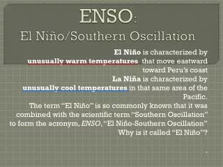
El Niño and La Niña events are defined by sea surface temperature anomalies in the Nino 3.4 region. Values are typically normalized by the standard deviation.
S.D.=0.83 S.D.=0.87 Control Observations
Wavelet analysis Power Spectrum: Averaged in time: Observations
S.D.=0.83 S.D.=0.87 Control Observations
LGM Values Normalized by Their standard Deviation 9,000 B.P. 6,000 B.P. Control Observations 2xCO2


![El Niño Southern Oscillation [ENSO]](https://cdn1.slideserve.com/1597810/el-ni-o-southern-oscillation-enso-dt.jpg)