Download

1 / 22
220 likes | 416 Views
Introduction to the Tightbinding (LCAO) Method. Tightbinding: 1 Dimensional Model #1. Consider an Infinite Linear Chain of identical atoms, with 1 s-orbital valence e - per atom & interatomic spacing = a

E N D
Tightbinding: 1 Dimensional Model #1 • Consider anInfinite Linear Chainof identical atoms, with 1 s-orbitalvalence e- per atom & interatomic spacing = a • Approximation:Only Nearest-Neighbor interactions.(Interactions between atoms further apart than a are ~ 0). This model is called the “Monatomic Chain”. n =Atomic Label a n =-3 -2 -1 0 1 2 3 4 Each atom has s electron orbitals only! Near-neighbor interaction only means that thesorbital on site ninteracts with the sorbitals on sites n – 1 & n + 1 only!
a • The periodic potential V(x) for this Monatomic Linear Chainof atoms looks qualitatively like this: n = -4 -3 -2 -1 0 1 2 3 V(x) = V(x + a)
a • The localized atomic orbitals on each site for this Monatomic Linear Chainof atoms look qualitatively like this: n = -4 -3 -2 -1 0 1 2 3 The spherically symmetric sorbitals on each site overlap slightly with those of their neighbors, as shown. This allows the electron on site n to interact with its nearest-neighbors on sites n – 1 & n + 1!
The True Hamiltonian in the solid is: H = (p)2/(2mo) + V(x), with V(x) = V(x + a). • Instead, approximate it as H ∑n Hat(n) + ∑n,nU(n,n) where, Hat(n) Atomic Hamiltonian for atom n. U(n,n) Interaction Energy between atoms n & n. Use the assumption of only nearest-neighbor interactions: U(n,n) = 0 unless n = n -1 or n = n +1 • With this assumption, the Approximate Hamiltonian is H ∑n [Hat(n) + U(n,n -1) + U(n,n + 1)]
H ∑n [Hat(n) + U(n,n -1) + U(n,n + 1)] • Goal:Calculate the bandstructure Ek by solving the Schrödinger Equation: HΨk(x) = Ek Ψk(x) • Use the LCAO(Tightbinding) Assumptions: 1. H is as above. 2. Solutions to the atomic Schrödinger Equation are known: Hat(n)ψn(x) = Enψn(x) 3. In our simple case of 1 s-orbital/atom: En= ε = the energy of the atomic e- (known) 4.ψn(x) is very localized around atom n 5. The Crucial (LCAO) assumption is: Ψk(x) ∑neiknaψn(x) That is, the Bloch Functions are linear combinations of atomic orbitals!
Dirac notation:Ek Ψk|H|Ψk (This Matrix Element is shorthand for a spatial integral!) • Using the assumptions for H & Ψk(x) already listed: Ek =Ψk|∑n Hat(n) |Ψk + Ψk|[∑nU(n,n-1) + U(n,n-1)]|Ψk also note that Hat(n)|ψn= ε|ψn • The LCAO assumption is:|Ψk∑neikna|ψn • Assume orthogonality of the atomic orbitals: ψn |ψn= δn,n (= 1, n = n; = 0, n n) • Nearest-neighbor interaction assumption: There is nearest-neighbor overlap energy only! (α = constant) ψn|U(n,n 1)|ψn - α; (n = n, & n = n 1) ψn|U(n,n 1)|ψn= 0, otherwise It can be shown that for α > 0, this must be negative!
As a student exercise, show that the “energy band” of this model is: Ek= ε - 2αcos(ka) or Ek = ε - 2α + 4α sin2[(½)ka] • A trig identity was used to get last form.ε&αare usually taken as parameters in the theory, instead of actually calculating them from the atomic ψn The “Bandstructure” for this monatomic chain with nearest-neighbor interactions only looks like (assuming 2α< ε): (ET Ek - ε + 2α) ET It’s interesting to note that: The form Ek= ε - 2αcos(ka) is similar to Krönig-Penney model results in the linear approximation for the messy transcendental function! There, we got: Ek = A - Bcos(ka) where A & B were constants. 4α
Tightbinding: 1 Dimensional Model #2 A1-dimensional “semiconductor”! • Consider anInfinite Linear Chainconsisting of 2 atom types, A & B (a crystal with 2-atom unit cells), 1 s-orbitalvalence e- per atom & unit cell repeat distance = a. • Approximation:Only Nearest-Neighbor interactions.(Interactions between atoms further apart than ~ (½ )a are ~ 0). This model is called the “Diatomic Chain”. A B A B A B A n = -1 0 1 a
The True Hamiltonian in the solid is: H = (p)2/(2mo) + V(x), with V(x) = V(x + a). • Instead, approximate it (with γ= A or =B) as H ∑γnHat(γ,n) + ∑γn,γnU(γ,n;γ,n) where, Hat(γ,n) Atomic Hamiltonian for atom γin celln. U(γ,n;γ,n) Interaction Energy between atom of type γ in celln & atom of type γ in cell n. Use the assumption of only nearest-neighbor interactions: The only non-zero U(γ,n;γ,n) are U(A,n;B,n-1) = U(B,n;A,n+1) U(n,n-1) U(n,n+1) • With this assumption, the Approximate Hamiltonian is: H ∑γnHat(γ,n) + ∑n[U(n,n -1) + U(n,n + 1)]
H ∑γnHat(γ,n) + ∑n[U(n,n -1) + U(n,n + 1)] • Goal:Calculate the bandstructure Ek by solving the Schrödinger Equation: HΨk(x) = EkΨk(x) • Use the LCAO(Tightbinding) Assumptions: 1. H is as above. 2. Solutions to the atomic Schrödinger Equation are known: Hat(γ,n)ψγn(x) = Eγnψγn(x) 3. In our simple case of 1 s-orbital/atom: EAn= εA= the energy of the atomic e- on atom A EBn= εB= the energy of the atomic e- on atom B 4.ψγn(x) is very localized near cell n 5. The Crucial (LCAO) assumption is: Ψk(x) ∑neikna∑γCγψγn(x) That is, the Bloch Functions are linear combinations of atomic orbitals! Note!! The Cγ’s are unknown
Dirac Notation:Schrödinger Equation: Ek Ψk|H|Ψk ψAn|H|Ψk = EkψAn|H|Ψk (1) • Manipulation of (1), using LCAO assumptions, gives (student exercise): εAeiknaCA+ μ[eik(n-1)a + eik(n+1)a]CB= EkeiknaCA(1a) • Similarly:ψBn|H|Ψk = EkψBn|H|Ψk (2) • Manipulation of (2), usingLCAO assumptions,gives (student exercise): εBeiknaCB+ μ[eik(n-1)a + eik(n+1)a]CA= EkeiknaCA(2a) Here, μψAn|U(n,n-1)|ψB,n-1ψBn|U(n,n+1)|ψA,n+1 = constant (nearest-neighbor overlap energy) analogous to αin the previous 1d model
Student exercise to show that these simplify to: 0 = (εA - Ek)CA + 2μcos(ka)CB, (3) and 0 = 2μcos(ka)CA + (εB - Ek)CB, (4) • εA,εB , μare usually taken as parameters in the theory, instead of computing them from the atomic ψγn • (3) & (4) are linear, homogeneous algebraic equations for CA& CB 22 determinant of coefficients = 0 • This gives: (εA - Ek)(εB - Ek) - 4 μ2[cos(ka)]2 = 0 A quadratic equation for Ek! 2 solutions: a “valence” band & a “conduction” band!
Results: “Bandstructure” of the Diatomic Linear Chain(2 bands): E(k) = (½)(εA + εB) [(¼)(εA - εB)2 + 4μ2 {cos(ka)}2] • This gives a k = 0 bandgap of EG= E+(0) - E-(0) = 2[(¼)(εA - εB)2 + 4μ2]½ • For simplicity, plot in the case 4μ2 << (¼)(εA - εB)2&εB> εA Expand the [ ….]½part ofE(k) & keep the lowest order term E+(k) εB + A[cos(ka)]2, E-(k) εA - A[cos(ka)]2 EG(0) εA – εB + 2A, where A (4μ2)/|εA - εB|
Tightbinding Method: 3 Dimensional Model • Model: Consider a monatomic solid, 3d, with only nearest-neighbor interactions. Hamiltonian: H = (p)2/(2mo) + V(r) V(r) = crystal potential, with the full lattice symmetry & periodicity. • Assume (R,R = lattice sites): H ∑RHat(R) + ∑R,RU(R,R) Hat(R) Atomic Hamiltonian for atom at R U(R,R) Interaction Potential between atoms at R & R Near-neighbor interactions only! U(R,R) = 0 unless R & Rare nearest-neighbors
Goal: Calculate the bandstructure Ek by solving the Schrödinger Equation: HΨk(r) = EkΨk(r) • Use the LCAO(Tightbinding) Assumptions: 1. H is as on previous page. 2. Solutions to the atomic Schrödinger Equation are known: Hat(R)ψn(R) = Enψn(R), n = Orbital Label (s, p, d,..), En= Atomic energy of the e- in orbital n 3.ψn(R) is very localized around R 4. The Crucial (LCAO) assumption is: Ψk(r) = ∑ReikR∑nbnψn(r-R) (bnto be determined) ψn(R): The atomic functions are orthogonal for different n & R That is, the Bloch Functions are linear combinations of atomic orbitals!
Dirac Notation:Solve the Schrödinger Equation: Ek Ψk|H|Ψk The LCAOassumption: |Ψk= ∑ReikR∑nbn|ψn(1) (bnto be determined) • Consider a particular orbital with label m: ψm|H|Ψk = Ekψm|H|Ψk (2) • Use (1) in (2). • Then use 1. The orthogonality of the atomic orbitals 2. The assumed form of H 3. The fact that ψn(R) is very localized around R 4. That we know the atomic solutions to Hat|ψn = En|ψn 5. The nearest neighbor assumption that U(R,R) = 0 unless R & R are nearest-neighors.
Manipulate (several pages of algebra) to get: (Ek - Em)bm+ ∑n∑R0 eikR γmn(R)bn = 0 , (I) where: γmn(R) ψm|U(0,R)|ψn “Overlap Energy Integral” • The γmn(R) are analogous to the α&μin the 1d models. They are similar to Vssσ, etc. in real materials, discussed next! The integrals are horrendous to do for real atomic ψm! In practice, they are treated as parameters to fit to experimental data. • Equation (I): Is a system of N homogeneous, linear, algebraic equations for the coefficients bn. N = number of atomic orbitals. • Equation (I) for N atomic states The solution is obtained by taking anN N determinant! This results in N bandswhich have their roots in the atomic orbitals! • If the γmn(R)are “small”, each band can be thought of as Ek ~ En + k dependent corrections That is, the bands are ~ atomic levels + corrections
Equation (I): A system of homogeneous, linear, algebraic equations for the bn • N atomic states Solve an N N determinant! N bands Note: We’ve implicitly assumed 1 atom/unit cell. If there are n atoms/unit cell, we get nN equations &nN bands! • Artificial Special Case #1: One s level per atom 1 (s-like) band • Artificial Special Case #2:Three p levels per atom 3 (p-like) bands • Artificial Special Case #3: One s and three p levels per atom & sp3 bonding 4 bands NOTE that For n atoms /unit cell, multiply by n to get the number of bands!
Back to: (Ek - Em)bm+ ∑n∑R0 eikR γmn(R)bn = 0 , (I) where:γmn(R) ψm|U(0,R)|ψn “Overlap Energy Integral” • Also:Assume nearest neighbor interactions only ∑R0is ONLYover nearest neighbors! • Artificial Special Case #1: One s level per atom 1 (s-like) band: Ek = Es - ∑R=nneikR γ(R) But γ(R)= γ is the same for all neighbors so: Ek = Es - γ∑R=nneikR • Assume, for example, a simple cubic lattice: Ek = Es -2γ[cos(kxa) + cos(kya) +cos(kza)]
Artificial Special Case #2: Three p levels per atom. Gives a 3 3 determinant to solve. 3 (p-like) bands Student exercise!! Artificial Special Case #3: One s and three p levels per atom & sp3 bonding Gives a 3 3 determinant to solve. 4 bands Student exercise!!