Download
1 / 18
180 likes | 186 Views
This study explores the use of remote sensing and GIS data for estimating water productivity in a large basin. It examines the current status, spatial variation, causes, and scope for improvement of basin water productivity. The study also includes remote sensing techniques for assessing land productivity, water consumption, cropped areas, and water resources in the basin.

E N D
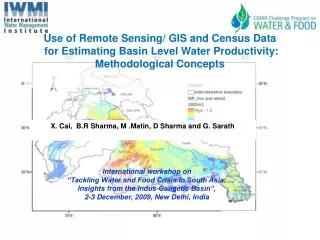
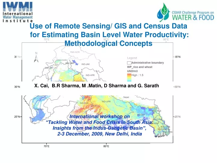
Use of Remote Sensing/ GIS and Census Data for Estimating Basin Level Water Productivity: Methodological Concepts X. Cai, B.R Sharma, M .Matin, D Sharma and G. Sarath International workshop on “Tackling Water and Food Crisis in South Asia: Insights from the Indus-Gangetic Basin”, 2-3 December, 2009, New Delhi, India
Basin focal project – Indo-Gangetic basin Basin fact sheet: Geographic Area: 2.25 million km2 Population: 747 million Landscape: mountain to plain Annual precipitation: 100 – 4000 mm Cropland area: 1.14million km2 Cropping pattern: rice–wheat Water use by agri.: 91.4% Water sources: ground water and surface water A basin under extreme pressure…
Basin Water Productivity Assessment – What to Care? • Magnitude – What’s the current status? • Spatial Variation – Hot spots/bright spots? • Causes – Why does WP vary (both high and low)? • Scope for improvement – How much potential for, where? • Irrigated vs. rainfed – What’s the option for sustainable development under water scarcity and food deficit conditions? • Crop vs. livestock and fisheries – How is livestock and fisheries contributing to water use outputs?
Basin Water Productivity Assessment – A Remote Sensing Perspective Land productivity – The natural extent of “good” and “bad” areas; Water consumption – How much water is depleted by what finally in spite of various ground conditions and interventions, and where (which drop for which crop)? Cropped areas – Cropping patterns and the spatial distribution; Water resources – Rainfall monitoring(TRMM); Factors assessment – Spatial analysis on causes for variations. Scope for improvement – “Hot Spots” / ”Bright Spots”
Remote Sensing for WP Assessment in Large Basin Areas – The Challenges The dynamic relation of spectra reflectance to crop biophysical characteristics; The often seen gaps in remote sensing interpretations to statistical data; The uncertainties in land surface parameterization for surface energy balance modeling.
Water Productivity Assessment Using Remote Sensing – The Five Steps • Crop Dominance Map • Crop Productivity Maps • Crop Consumptive Water Use • Water Productivity and the Variations • Causes for Variations and Scope for Improvement
Dataset • Census data: District wise crop area, yield and production, state wise livestock and fisheries production; • Satellite sensor data:Moderate Resolution Imaging Spectror-adiometer (MODIS) 250m 16 day Normalized Difference Vegetation Index (NDVI) mosaic of the basin, MODIS 1km 16 day Land Surface Temperature (LST) products: Nov 2005 – Oct 2006; • Weather data: Daily temperature, humidity, sea level pressure, precipitation, wind speed collected for 58 stations: 2005 – 2007; • Land Use Land Cover (LULC) maps: USGS GLC 1992-93, IWMI IG basin LULC map 2005, IWMI GIAM 10km (1999) and 500m (2003); • Other data layers: Basin boundary, administrative boundaries, road, railway, and river networks, Digital Elevation Model(DEM) • Ground truth data: see continued… To use all kinds of available information for the purpose of large scale WP assessment.
Ground truth A ground truth mission was conducted in India from 8th -17th Oct, 2008 • Across Indus and Gangetic river basin • >2700km covered • 175 samples • LULC • Cropping pattern • Agricultural productivity (cut and farmer survey) • Water use (rainfed, surface/GW) • Social-economic survey
Crop Dominance Map Synthesizing existing maps to a crop dominance map with GT data 500m, IWMI, 2003 (Base map) 500m, IWMI, 2005 1km, USGS, 1992-1993
Crop Dominance Map Predominant crops: irrigated rice/rice-wheat rotation Crop coefficients of the basin as extracted from literature (values) and RS imagery (growth periods) The predominant crops are mainly cultivated in a belt along the main streams of Ganges and Indus river.
Crop productivity Step 1. District wise productivity map using census data Crop GVP map of India and Nepal for 2005 Kharif season IGB paddy rice yield map of 2005 The approach is illustrated for rice, wheat is also done in the same way
Crop productivity Step 2. Pixel wise rice productivity map interpolation using MODIS data NDVI composition of 29 Aug – 5 Sept 2005 for rice area paddy rice yield map of 2005 MODIS 250m NDVI at rice heading stage was used to interpolate yield from district average to pixel wise employing rice yield ~ NDVI linear relationship.
Actual ET estimation Step 1. Potential ET calculation (2005-09-21 as example) Daily data from 58 weather stations potential ET map (2005 Sept 21) • Steps: • Hargreaves equation for reference ET. • Kc approach for potential ET. • Note: Kc (FAO56) was determined by maximum Kc values of major crop of the month
SSEB ETa– the actual Evapotranspiration, mm. ETf – the evaporative fraction, 0-1, unitless. ET0 – Potential ET, mm. Tx– the Land Surface Temperature (LST) of pixel x from thermal data. TH/TC– the LST of hottest/coldest pixels. Actual ET estimation Step 2. Actual ET calculation by Simplified Surface Energy Balance (SSEB) approach MODIS LST 2005 Sept 21 ET fraction map (2005 Sept 21) potential ET map (2005 Sept 21) Seasonal actual ET map (2005 Jun 10 – Oct 15)
Rice yield and ETa maps Huge variation in yield, indicating significant scope for improvement ET is high where yield is high. However, ET might also be high where yield is not (so) high. Why? Yield (ton/ha) ETa (mm)
Wheat yield and ETa maps Huge variation in yield, indicating significant scope for improvement ETa (mm) Wheat ET variation is more consistent with yield Yield (ton/ha)
Water productivity maps Rice (kg/m3) Wheat (kg/m3) Note: 1% of the points with extremely low and high values are sieved from the statistics