Download

1 / 21
210 likes | 281 Views
Measuring Welfare Changes of Individuals. Exact Utility Indicators Equivalent Variation (EV) Compensating Variation (CV) Relationship between Exact Utility Indicators and Consumer Surplus (CS) How accurate an approximation of utility change is CS? See Zerbe and Dively, Chapter 5.

E N D
Measuring Welfare Changes of Individuals • Exact Utility Indicators • Equivalent Variation (EV) • Compensating Variation (CV) • Relationship between Exact Utility Indicators and Consumer Surplus (CS) • How accurate an approximation of utility change is CS? See Zerbe and Dively, Chapter 5
Money Measure of Individual Utility • Each indifference curve of an individual consumer corresponds to a unique level of income • If prices are fixed! • The change in utility of an individual from a policy that provides a direct cash transfer, without changing any prices, can be measured by the value of the transfer
Indifference Curves X2 M2 M1 M0 U3 U2 U1 U0 X1
Equivalent Variation • Consider an action which will cause a price to change. • This price change will change the utility of the consumer
Equivalent Variation • How much money would have to be given to or taken away from the consumer to give them the equivalentutility of the proposed action. • Consumer moves to new utility level, but the action not undertaken (prices do not change)
Equivalent Variation Y EV U1 U0 P1 P0 X
Compensating Variation • After introducing a change, how much money would have to be given to or taken away from a consumer (compensation) to place them at their original level of utility • Action is undertaken but income provided to or taken away to place the consumer at the previous level of utility. (prices do change)
Compensating Variation Y CV U1 U0 P1 P0 X
Equivalence of EV and CV EV for price decrease = CV for price increase CV for price decrease = EV for price increase
EV for a Price Decrease Y EV U1 U0 P1 P0 X
CV for a Price Increase Y CV U0 U1 P0 P1 X
Marshallian vs Hicksian Demand Curves • Marshallian demand curve: • Shows quantities demanded for different price levels, holding money income constant. • Slutsky decomposition of effect of a price change: • Pure substitution effect • Income effect
Marshallian vs Hicksian Demand Curves • Hicksian, or compensated demand curve • Shows quantities demanded at different price levels, holding utility constant. • Only the pure substitution effect • Smaller response to price change (less elastic), than Marshallian demand curve - for normal goods.
Marshallian and Hicksian Demand Curves Y Price decrease U1 U0 P1 P0 X X0 X1H X1M
Marshallian and Hicksian Demand Curves Price decrease Px P0 x P1 x x DM DH X0 X1H X1M Qx
Marshallian and Hicksian Demand Curves Y Price Increase U0 U1 P0 P1 X X1M X1H X0
Marshallian and Hicksian Demand Curves Price Increase Px P1 x x P0 x DM DH X1M X1H X0 Qx
Marshallian and Hicksian Demand Curves Px P1 P0 DM DH|U(P1) DH|U(P0) Qx
CV, EV, & CS • CV and EV are measured on Hicksian (compensated) demand curves • CS is measured on Marshallian demand curve • CS is only approximation of welfare change • It is “average between CV and EV • Willig – under wide range of conditions CS is close approximation of CV, EV.
Marshallian and Hicksian Demand Curves Px P1 CV EV CS P0 DM DH|U(P1) DH|U(P0) Qx
Comparison of CS, EV CV • Empirically, we are able to estimate CS, but not EV or CV. • How close an approximation is CS to EV or CV? • Depends on magnitude of the income effect • Differences are small for small price changes • Differences are small if (Marshallian) demand curve is inelastic