Download
1 / 27
290 likes | 1.03k Views
Phasor-Domain Equations. Transmission line equations — time domain: Time domain Phasor domain. Transmission line equations — phasor domain:. Phasor-Domain Equations. Advantages of Phasor-Domain Representation

E N D
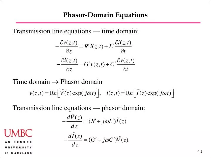
Phasor-Domain Equations Transmission line equations — time domain: Time domain Phasor domain Transmission line equations — phasor domain:
Phasor-Domain Equations • Advantages of Phasor-Domain Representation • Reduction from partial differential equation to ordinary differential equation — so that it is easier to solve • Allows generalization: • Advantages of Time-Domain Representation • Allows study of transients
Phasor-Domain Equations • Second-Order Equations: • with g = complex propagation constant a = Re(g ) = attenuation constant (Np/m) b = Im(g ) = phase constant or wavenumber (rad/m) NOTES: We pick a and b so that both are positive In a passive medium, a is always positive; it can be negative in an active medium [An active medium, like a laser, has an energy source; a passive medium does not and must always lose energy.]
Phasor-Domain Equations • The second-order equations have the general solutions • are not independent • We may also write: where is the characteristic impedance NOTE: Z0 (Ulaby’s notation) ZC (Paul’s notation)
Phasor-Domain Equations • Returning to the time domain: • We first write • from which we obtain Phase velocity = up = w/b
Phasor-Domain Equations Example: Ulaby Exercise 2.4Question: A two-wire air line has the following parameters: R′ = 0.404 m/m, L′ = 2.00 mH/m, G′ = 0, C′ = 5.56 pF/m. For operation at 5 kHz, determine (a) the attenuation coefficient a, (b) the wavenumber b, (c) the phase velocity up, and the characteristic impedance Z0. Answer:w = 2 × 3.14159 × (5×103 s–1) = 3.14159×10⁴ s–1. R′ + jwL′ = (4.04000×10⁻⁴ + j×3.14159×104 × 2.00000×10–6 ) /m = (4.04000×10⁻⁴ + j×6.28318×10⁻² ) /m = 6.28319×10⁻² × exp( j×1.56436) /m . G′ + jwC′ = j×1.74673×10⁻⁷ –1/m = 1.74673×10⁻⁷ × exp( j×1.57080) –1/m. Note the small difference in phases! Six digits of accuracy are needed to keep three digits in the attenuation coefficient. g 2 = 1.09750×10⁻⁸ × exp( j×3.13156) m–2, so that g = 1.04762×10⁻⁴ × exp( j×1.56758) m–1 = 3.37×10⁻⁷ + j×1.04761×10⁻⁴, so that • = 3.37×10⁻⁷ Np/m and b = 1.05×10⁻⁴ rad/m. We have up = w / b = (3.142/1.048) ×108 = 3.00 ×10⁸ m/sand Z0 = {(6.283×10⁻² / 1.747×10⁻⁷ ) exp[ j×(1.56436 – 1.57080)]}1/2 = (600 – j×1.93) W
Lossless Transmission Line • Specializing to the case of no loss (R′ = 0, G′ = 0 ): • We will later show that for any TEM transmission line: m = magnetic permeability e = electrical permittivity • For any insulating material that would be used in a transmission line, , where m0 is the vacuum permeability. — The value for m0 is exact and defines the relation between B and H. • By contrast, the values for e differ significantly for different materials. We write: e = er e0, where er is referred to as the relative permittivity, and is the vacuum permittivity
Lossless Transmission Line • We now have: • In optics, we define an index of refraction, n = c / up, so that
Lossless Transmission Line Coaxial Two wire Parallel plane K • The impedance relation: • is a bit more complex. It involves a geometric factor K. The vacuum impedance of 377W is a very important number • Loads with lower impedance have large magnetic near fields • Loads with higher impedance have large electric near fields • EMI properties are very different in the two cases! Table of Geometric Factor K
Lossless Transmission Line Voltage Reflection: When a = 0, our phasor relations become At the load, we have which implies and defines the voltage reflection coefficient G Load impedances and reflection coefficients are usually complex!
Lossless Transmission Line Example: Ulaby Exercise 2.7Question: A 50 lossless transmission line is terminated in a load impedance ZL = (30 – j200) . Calculate the voltage reflection coefficient at the load. Answer: G = (ZL – Z0 ) / (ZL + Z0 ) = (30 – j200 – 50) / (30 – j 200 + 50) = (–20 – j200) / (80 – j 200) = 201exp(– j1.67) / 215exp (– j1.19)= 0.93exp (– j0.48). NOTE: – 0.48 rads = – 28o. Writing G = |G| exp ( jqr) , we find qr = – 0.48 rads.
Lossless Transmission Line • Standing Waves • After using the relation in the phasor equations, • We then find • so that the amplitude of the voltage varies sinusoidally with z. • This pattern is called a standing wave. • It comes from the interference of forward- and backward- propagating waves
Lossless Transmission Line • Standing Waves • The voltage and current maxima and minima are 180o out of phase • The amplitude multiplies a cos(wt) dependence with a complicated but periodicz-variation. • The maxima and minima are spaced l / 2 apart Ulaby Figure 2-11 Figure Parameters: |G| = 0.3, qr = 30o Z0 = 50 W
Lossless Transmission Line • Standing Waves • The total dependence of the standing wave voltage is Ulaby 2001 CD
Lossless Transmission Line • Standing Waves • For a matched load (ZL = Z0), there is no standing wave • For a short-circuited load (ZL = 0) or an open-circuited load (ZL = ), there are complete reflections and an oscillation depth of 100% • With |G| = 1, there are points where the voltage is exactly zero, spaced l / 2 apart Ulaby Figure 2-12
Lossless Transmission Line • Standing Waves • We will designate the location of the maxima as lmax = –z, so thatlmax is a positive number (since the load is at z = 0). Only n-values that satisfy lmax 0 are allowed • The voltage standing wave ratio (VSWR or SWR) gives the gives the oscillation depth. It is defined:
Lossless Transmission Line Example: UlabyExercise 2.11Question: A 140 lossless line is terminated in a load impedance ZL = (280 + j182) . If l = 72 cm, find (a) the reflection coefficient G, (b) the VSWR S, (c) the locations of the voltage maxima and minima. Answer: (a)G = (ZL – Z0 ) / (ZL + Z0 ) = (280 + j182 – 140) / (280 + j 182 + 140) = 230 exp( j0.915) / 458exp (j0.409) = 0.50exp ( j0.51). NOTE: 0.51 rads = 29o. (b) S = (1 + |G|) / (1 – |G|) = (1 + 0.502) / (1 – 0.502) = 3.0. (c) lmax = (0.506 × 72 / 4p + n × 72 / 2) cm = 2.9 cm, 39 cm, 75 cm,…; lmin = (0.506 × 72 / 4p + 18 + n × 72 / 2) cm = 21 cm, 57 cm, 93 cm,…
Lossless Transmission Line Input Impedance With standing waves, the voltage-to-current ratio, which is referred to as the input impedance, varies as a function of position Of particular interest is the input impedance at the generator, z = –l
Lossless Transmission Line Input Impedance From the standpoint of the generator circuit, the transmission line appears as an input impedance , so that From the standpoint of the transmission line Combining these relations… Ulaby Figure 2-14
Lossless Transmission Line Input Impedance …we conclude Thus, we can now relate the wave parameters, to the transmission line parameters and the input parameters
Lossless Transmission Line L Paul Example 6.7 (extended)Question: A line 2.7 m in length is excited by a 100 MHz source asshown in the figure. Determine the source and load voltages. Determine the voltages and the current everywhere in the transmission line Answer: We will work in Ulaby’s notation, and our first task is to translate Paul’s problem specification into that notation: Paul Figure 6.21
Lossless Transmission Line Paul Example 6.7Answer (continued):* (1) Find the reflection coefficient: (2) Find the propagation factor *NOTE: I am using MATLAB to calculate values. So, the calculations are good to15 places, although I only report three.
Lossless Transmission Line Paul Example 6.7Answer (continued): (3) Find the input impedance:
Lossless Transmission Line Paul Example 6.7Answer (continued): (4) Find the input voltage:
Lossless Transmission Line Paul Example 6.7Answer (continued): (5) Find the load voltage:
Lossless Transmission Line Paul Example 6.7Answer (continued): (6) Write the time domain voltages: (7) Find the phasor domain voltage and current in the transmission line
Lossless Transmission Line Paul Example 6.7Answer (continued): (8) Find the time domain voltage and current in the transmission line: (9) Checks: