Download
1 / 26
270 likes | 550 Views
Lecture 5: Uniprocessor Scheduling. Advanced Operating System Fall 2010. Contents. Basic Concepts Scheduling Criteria Scheduling Algorithms Uniprocessor scheduling – multilevel queue scheduling. Basic Concepts.

E N D
Lecture 5: Uniprocessor Scheduling Advanced Operating System Fall 2010
Contents • Basic Concepts • Scheduling Criteria • Scheduling Algorithms • Uniprocessor scheduling – multilevel queue scheduling
Basic Concepts • Scheduling is concerned with the decision of assigning processor (or processors) to processes in such a way so as to optimize a number of performance criteria. These performance criteria can be user-oriented or system-oriented. • Types of Scheduling • Long-term scheduling – the decision to add to the pool of processes to be executed. • Medium-term scheduling – The decision to add to the number of processes that are partially or full in main memory. • Short-term scheduling – The decision as to which available process will be executed by the processor. • I/O scheduling – The decision as to which process’ pending I/O request shall be handled by the available I/O device. • The first 3 types of scheduling are processor scheduling. The last one is a function of the characteristic of the I/O device – e.g. disk or tape. • We shall discuss about the first 3 types.
Long-Term Scheduling • The long-term scheduling determines which programs are admitted to the system for processing. Thus, it controls the degree of multiprogramming. • For interactive programs in a time-sharing system, a process request can be generated by the act of a user attempting to connect to the system. The OS will accept all authorized users until the system is saturated, using some predefined measure of saturation. Once the predefined measure of saturation is reached, the next request will be blocked with a message that the system is full and the user should try again later. • In a batch system, a newly submitted job is first routed to a disk. The long-term scheduler decides when to admit the new job into the system. There are 2 decisions involved here: • The long-term scheduler must decide when to take on an additional job. • Which job (or jobs) to choose.
Long-Term Scheduling (cont.) • For decision 1. the decision is driven by the desired degree of multiprogramming. The degree of multiprogramming is dictated by the available resources (e.g. enough memory. • For decision 2, the decision can be on a FCFS policy, or certain criteria based on priority, expected execution time, or I/O requirements. For example, the scheduler may attempt to keep a mix of processor-bound and I/O-bound processes. The scheduler may attempt to keep a good mix of short jobs (student jobs) and long jobs (research projects)
Medium-term scheduling • Medium-term scheduling is part of the swap-out function. Typically, blocked processes are the ones to swap-out. It is a function of the desired degree of multiprogramming as well as the cost of swapping.
Short-term scheduling(dispatcher) • The short-term scheduler is invoked whenever an event occurs that may lead to the suspension of the current process or that may provide an opportunity to preempt a currently running process in favor of another. Examples of such events include the following: • Clock interrupts • I/O interrupts • OS calls • Signals
Dispatcher • Dispatcher module gives control of the CPU to the process selected by the short-term scheduler; this involves: • switching context • switching to user mode • jumping to the proper location in the user program to restart that program • Dispatch latency – time it takes for the dispatcher to stop one process and start another running
Short-term Scheduling Criteria • System-Oriented Criteria • CPU utilization – percentage time that the processor is busy, keep the CPU as busy as possible (maximize processor utilization) • Throughput – # of processes that complete their execution per time unit (maximize throughput) • User-Oriented Criteria • Turnaround time – interval of time between submission of a job and its completion, i.e., the total time that the process spends in the system (waiting time plus service time). Appropriate measure for batch job. • Waiting time – amount of time a process has been waiting in the ready queue • Response time – amount of time it takes from when a request was submitted until the first response is produced, not output (for time-sharing environment) • Deadline – The ability to meet hard deadline. Appropriate for real-time jobs
Short-term SchedulingCPU Scheduler • Selects from among the processes in memory that are ready to execute, and allocates the CPU to one of them • Scheduling Discipline: • Nonpreemptive – Once a process is in the Running State, it continues to execute until • (a) it terminates • (b) blocks itself to wait for I/O or to request some OS services • Preemptive – The currently running process may be interrupted and moved to the Ready State by the OS • (a) Switches from running to ready state • (b) Switches from waiting to ready state • Preemptive more overhead than nonpreemptive, but may provide better service
Optimization Criteria • Max CPU utilization • Max throughput • Min turnaround time • Min waiting time • Min response time
Scheduling Algorithm • Turnaround Time(TAT) is the total time that the process spends in the system (waiting time + service time). • Normalized Turnaround Time is the ratio of Turnaround Time to Service Time
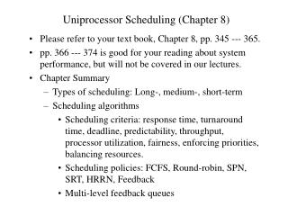
D A E B C 9 0 13 18 20 3 First-Come, First-Served (FCFS) Scheduling ProcessArrival TimeService Time A 0 3 B 2 6 C 4 4 D 6 5 E 8 2 • The Gantt Chart for the schedule is: • Turnaround Time(TAT) A: 3; B: 7; C: 9; D: 12; E: 12 • Normalized Turnaround Time: A: 3/3=1.0; B: 7/6; C: 9/4=2.25; D: 12/5=2.4; E: 12/2=6.0
Round Robin (RR) • Used in interactive time-sharing system. • Each process gets a small unit of CPU time (time quantum), usually 10-100 milliseconds. After this time has elapsed, the process is preempted and added to the end of the ready queue. • If there are n processes in the ready queue and the time quantum is q, then each process gets 1/n of the CPU time in chunks of at most q time units at once. No process waits more than (n-1)q time units. • Performance • q large FIFO • q small processor sharing • q must be large with respect to context switch, otherwise overhead is too high • Best choice q for will be slightly greater than the time required for a typical interaction.
A A A B B C B C D B C E D B C D E B D 0 1 2 3 4 5 6 7 8 9 10 11 12 13 14 15 16 17 18 19 Example of RR with Time Quantum = 1 ProcessArrival TimeService Time A 0 3 B 2 6 C 4 4 D 6 5 E 8 2 The Gantt chart is: • Turnaround Time(TAT) A: 3; B: 16; C: 11; D: 14; E: 10 • Normalized Turnaround Time: A: 3/3=1.0; B: 16/6=8/3=2.66; C: 11/4=2.75; D: 14/5=2.8; E: 10/2=5
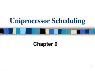
C A D B E 9 0 11 15 20 3 Shortest- Process-Next (SPN) Scheduling • This is a nonpreemptive scheduling discipline in which the shortest expected processing time is selected next. ProcessArrival TimeService Time A 0 3 B 2 6 C 4 4 D 6 5 E 8 2 The Gantt chart is: • Turnaround Time(TAT) A: 3; B: 7; E: 3; C: 11; D: 14 • Normalized Turnaround Time: A: 3/3=1; B: 7/6; E: 3/2; C: 11/4; D: 14/5 • Needs user to provide an estimate of processing time.
Determining Length of Next CPU Burst (not required) • For interactive processes, the OS may keep a running average of each “burst” for each process and estimate the processing time requirement of the next burst by • Ti= processor execution time for the ith instance of this process • Si= predicted value for the ith instance • S1=predicted value for the 1st instance, not calculated, assumed to be 0. • The equation can be rewritten as • The above formular gives equal weight to each instance. If we want to give greater weight to more recent instances, then we can use an exponential averaging where α is a constant and 0< α <1, • Because both α and (1- α) are less than 1, each successive term in the preceding equation is smalle. • The larger the value of α, the greater the weight given to the more recent observations.
Shortest Remaining Time(SRT) • It is a preemptive version of SPN. The scheduler always chooses the process that has the shortest expected remaining processing time. ProcessArrival TimeService Time A 0 3 B 2 6 C 4 4 D 6 5 E 8 2 The Gantt chart is: • Turnaround Time(TAT) A: 3; B: 13; C: 4; D: 14; E: 2 • Normalized Turnaround Time: A: 3/3=1; B: 13/6; C: 4/4=1; D: 14/5=2.8; E: 2/2=1 A B C E B D 15 20 0 3 4 8 10
Priority Scheduling • A priority number (integer) is associated with each process • The CPU is allocated to the process with the highest priority (smallest integer highest priority) • Preemptive • nonpreemptive • SJF is a priority scheduling where priority is the predicted next CPU burst time • FCFS is a priority scheduling where priority is the arrival time of the process. • Problem Starvation – low priority processes may never execute • Solution Aging – as time progresses increase the priority of the process
E A D B C 9 0 13 15 20 3 Highest Response Ratio Next • w= time spent waiting for the processor • s= expected service time • R=(w+s)/s • When a process is free for assignment, choose the process with the greatest value of R. ProcessArrival TimeService Time A 0 3 B 2 6 C 4 4 D 6 5 E 8 2 The Gantt chart is: • Calculate R: • at time 9: C: ((9-4)+4)/4=9/4; D: ((9-6)+5)/5=8/5; E: ((9-8)+2)/2=3/2, choose C • At time 13: D: ((13-6)+5)/5=2.4; E: ((13-8)+2)/2=3.5; choose E.
Multilevel Queue • Ready queue is partitioned into separate queues:foreground (interactive)background (batch) • Each queue has its own scheduling algorithm • foreground – RR • background – FCFS • Scheduling must be done between the queues • Fixed priority scheduling; (i.e., serve all from foreground then from background). Possibility of starvation. • Time slice – each queue gets a certain amount of CPU time which it can schedule amongst its processes; i.e., 80% to foreground in RR, 20% to background in FCFS
Multilevel Feedback Queue • A process can move between the various queues; aging can be implemented this way • Multilevel-feedback-queue scheduler defined by the following parameters: • number of queues • scheduling algorithms for each queue • method used to determine when to upgrade a process • method used to determine when to demote a process • method used to determine which queue a process will enter when that process needs service
Example of Multilevel Feedback Queue • Three queues: • Q0 – RR with time quantum 8 milliseconds • Q1 – RR time quantum 16 milliseconds • Q2 – FCFS • Scheduling • A new job enters queue Q0which is servedFCFS. When it gains CPU, job receives 8 milliseconds. If it does not finish in 8 milliseconds, job is moved to queue Q1. • At Q1 job is again served FCFS and receives 16 additional milliseconds. If it still does not complete, it is preempted and moved to queue Q2.
End of lecture 5 Thank you!