Download
1 / 14
140 likes | 326 Views
SEG 3-D Elastic Salt Model. Biondo Biondi, Bee Bednar, Arthur Chang leading SEG committee work John Anderson is XOM contact Meeting to discuss desirable features Thursday, June 23, 2005, GW3-933 9:00 am to 10:30 am Computational effort will take a long time

E N D
SEG 3-D Elastic Salt Model • Biondo Biondi, Bee Bednar, Arthur Chang leading SEG committee work • John Anderson is XOM contact • Meeting to discuss desirable features • Thursday, June 23, 2005, GW3-933 • 9:00 am to 10:30 am • Computational effort will take a long time • Current task is to define a suitable model
3-D SEG Acoustic Salt Model snap shot at 781 ms source snap shot at 1450 ms
45 shot data set 5 lines 9 shots/line 201 by 201 receiver grid per shot (40 m spacing, wide azimuth, source at center of grid, 40401 receivers/shot) ideal for shot record migration 4800 shot data(C3-NA) 50 lines, 160 m cross-line spacing 96 shots / line, 80 m shot spacing 8 cables, 40 m group interval within a cable 68 receivers / cable 544 receivers / shot simulates marine acquisition Acoustic (18 Hz peak)SEG Salt model (2 data sets)
Single raw 3-D shot record (8 streamers, C3-NA) Numerical dispersion Original SEG SALT model data Each streamer has 68 receivers 40 m apart. The entire survey is 50 lines with 96 shots per line. Time sample rate is 0.008 s, with 625 samples per trace
Computational Size of Problem • For 3-D acoustic SEG Salt model • Using model parameters for data without dispersion • 441 shot wide-azimuth data set • 21 lines of 21 shots each, receivers at every grid point • 650 GB if SEGY, 400 CPU days on old hardware • Aimed at ideal conditions for shot migration • For 3-D elastic model (similar to acoustic model) • scale compute time by roughly 144 • Vs = 0.5 Vp requires finer grid by factor of 2 • Computation time scale factor is 16=24 • 3 components x 3 terms = factor of 9 • Data set volume grows by factor of 3 • Doubling bandwidth requires factor of 16=24
Marmousi II 2-D Elastic Model (University of Houston) Vp Low p-wave velocity simulating hydrocarbons to give AVO response Flat spot on target Vs AVO modeling requires Vp, Vs, and Density Density Synthetic data have 80 Hz bandwidth
SEG 3-D Elastic Salt Model Key desirable features: (1) smooth and rugose (both deep notches and chirp signal) Top of Salt (TOS) components (2) shallow salt with impedance match to give large P-S conversions (3) deeper salt matched for P-P (4) multiple salt bodies, one obscuring portions of the other (5) compaction model for subsalt region honoring differences between salt and sediment overburdens
SEG 3-D Elastic Salt Model Key desirable features: (6) overpressure zone for part of subsalt zone (7) sediment profile with some AVO target anomalies (8) reservoir zones with compartmentalization (9) variations in the Base Of Salt (BOS) (steep ramp to flat, gentle ramp to flat) (10) subsalt sediments that truncate steeply against the BOS
SEG 3-D Elastic Salt Model Key desirable features: (11) realistic salt tectonics including faulting and structures in the sediments corresponding to deep salt withdrawal and slip interfaces (12) deep carbonate with rift faults near bottom of section. (13) components for calibrating image quality deep horizontal reflector at bottom isolated point diffractors
Sediment structures are related to salt tectonics Allochthonous Salt Autochthonous Salt
Salt Salt Autochthonous salt weld
Realistic Plan • Begin with a fully elastic model, progress as compute capacity grows • Acoustic model data set • Elastic multicomponent data set • Anisotropic multicomponent data set • Begin collecting data over subsets of the model • Subsets of the model could target different geologic objectives • Over time merge surveys to cover entire model • Surface, OBC, and VSP data • Both absorbing and reflecting surface boundary conditions • Zones of very dense sampling • Could we have an equivalent physical model done at Delft or University of Houston or elsewhere? • Can we get elastic physical models?