Download
1 / 37
370 likes | 496 Views
András Zénó Gyöngyösi, Tamás Weidinger, László Haszpra, Zsuzsanna Iványi and Hiroaki Kondo. Sensitivity Study of a Coupled Carbon Dioxide Meteorological Modeling System with Case Studies. The NIRE CO2 @ ETA model. Overview. Short model description NIRE ETA Implementation NIRE ETA

E N D
András Zénó Gyöngyösi, Tamás Weidinger, László Haszpra, Zsuzsanna Iványi and Hiroaki Kondo Sensitivity Study of a Coupled Carbon Dioxide Meteorological Modeling System with Case Studies The NIRE CO2 @ ETA model
Overview • Short model description • NIRE • ETA • Implementation • NIRE • ETA • Coupling of NIRE to ETA • Sensitivity studies • Case studies • Conclusion, future works
Model Description • NIRE • Mesoscale circulation model (simple dynamics) • Dispersion model • Boussinesq-approximation • Anelastic equations • Terrain following s-coordinate (vrbl. res.) • Staggered (Arakawa) grid • First order turbulent closure (K ~ Richardson #) • Vertical diff – implicit solver • Horizontal diff – just for numerical stability • Srfc: Monin-Obuhov; Energy Balance Eq. • Soil: Thermal conductivity eq.
Surface parameterization H2O: passive scalar, saturation @ srfc • No clouds, relevant in sfc heat balance CO2: • Vegetation (Photosynth.+Res.) for each veg. mosaic => synthesized flux • Anthropogen: • area sources @ srfc (heating and traffic) • large stacks – plume rise (CONCAWE)
Boundary conditioning; Numerical integration • Lateral bndry • Flow relaxation zone • Top bndry • Sponge layer • Initialization • Dynamical init. – spin-up • Time integration: Leap frog – Forward each 20th step to adjust numerical mode
Implementation • Surface files • IGBP landcover landuse database (USGS) • Sensitivity test • Dynamics • Superadiabatic stratification • Strong wind • Basin • Carpathian Basin @ bndry: nonlinear interaction topography -- bndry
Model bndry interacts w/ topography – strong nonlinear effects More effective bndry conditions are necessary
Sensitivity Study Mixing layer depth (Convective PBL)@ different cloud amounts Time evolution of CO2 in the model domain
The “Meteorological driver” • NCEP/ETA model (EMS NWS/NOAA): • Limited area NWP model • Primitive hydrostatic eqs – non-hydrost. Option • Modified terrain following coordinate system • Eta (modified sigma) • approx horiz. srfs separatio nof lee flow • sfc & PBL param. sophisticated
Adaptation of ETA Adaptation • ”Operational” run for Central Europe • “Operational” run for Central Europe + Budapest Init & bndry conds downloaded from NCEP every morning
Dynamical Test (non-hydrostatic option) • Hydrostatic equations, non-hydrostatic effects parameterized • Small-scale effect are more non-hydrost. • Small impact on solutions • In the standard run non-hydrost. Option not implemented • DF init. not used
The Mass field Pressure falling (approaching system) NH departure 9m Psfc H500 ∆h~-.4—1.4 h~5530—5620
The Wind field NH wind stronger more KE generation NH departures associated with topography
Coupling NIRE to ETA • Super-adiabatic lapse rate instab • Extreme wind speed • instab @ lat & top bndry • Flow relax term • changed to sine shape • Top sponge layer enlarged • Adiabat. adjustment:
A Case study • Cold inversion in the Basin 02 February 2006 “Inversion case” • Convective boundary layer after the decay of the inversion 06 February 2006 “Convection case”
Effect of a single large stack Plume rise (CONCAWE – Briggs, 1968) 200 m high 280 m3/s @ 3000C 1000 t/day CO2 emission Located in the middle of the domain
Time evolution of temperature Inversion Convection
Temperature Profiles @ different time of the day Inversion Convection
Time evolution of CO2 Inversion Convection
CO2 Profiles @ different time of the day Inversion Convection
Conclusion • NIRE is able to provide realistic meteorological conditions in suitable initial and boundary conditions taken from ETA • The modular structure of it makes them suitable for PBL tests • The coupled system is able to calculate concentration for different extreme meteorological conditions
Future works • Introduction of newer parameterization schemes into the CO2 model – further sensitivity and case studies • Daily coupled system runs for the estimation of annual variation of surface fluxes • Estimation of annual Carbon budget of the Carpatian Basin