Download
1 / 47
470 likes | 568 Views
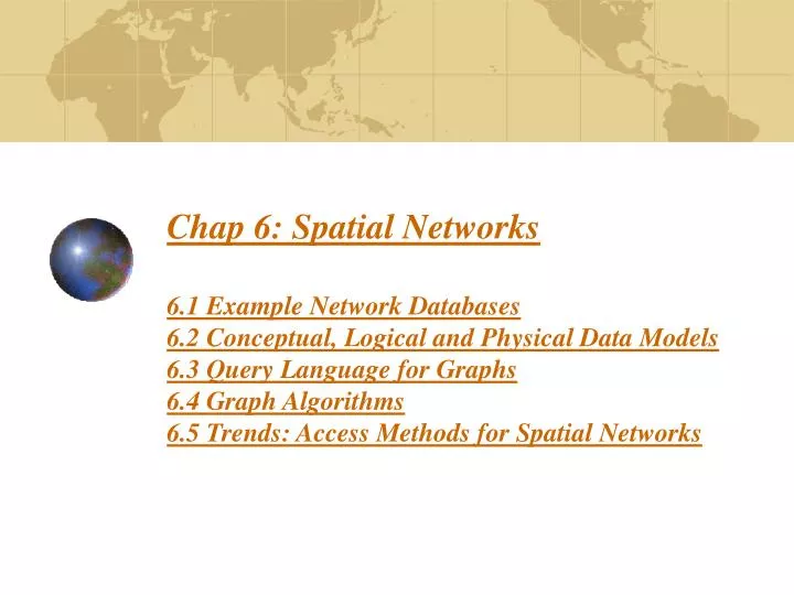
Chap 6: Spatial Networks 6.1 Example Network Databases 6.2 Conceptual, Logical and Physical Data Models 6.3 Query Language for Graphs 6.4 Graph Algorithms 6.5 Trends: Access Methods for Spatial Networks. Learning Objectives. Learning Objectives (LO)

E N D
Chap 6: Spatial Networks6.1 Example Network Databases6.2 Conceptual, Logical and Physical Data Models6.3 Query Language for Graphs6.4 Graph Algorithms6.5 Trends: Access Methods for Spatial Networks
Learning Objectives • Learning Objectives (LO) • LO1: Understand the concept of spatial network (SN) • What is a spatial network? • Why learn about spatial network? • LO2 : Learn about data models for SN • LO3: Learn about query languages and query processing • LO4: Learn about trends • Focus on concepts not procedures! • Mapping Sections to learning objectives • LO1 - 6.1 • LO2 - 6.2 • LO3 - 6.3, 6.4 • LO4 - 6.5
Motivation: Navigation Systems • In-vehicle navigation systems • Offered on many luxury cars • Services: • map destination given a street address • compute the shortest route to a destination • Help drivers follow selected route • Recall that many maps and GIS were made for navigation • 16th century shipping, trade and treasure hunts • Maps were used to find destination and avoid hazards • Navigation and transportation are important applications! • Can OGIS spatial abstract data types support navigation?
Navigation Systems and OGIS Spatial ADTs • Can OGIS spatial abstract data types support navigation? • OGIS spatial ADTs discussed in chapter 2 and 3 are inadequate for • computing route to a destination • Rationale: Part 1 • Fact: Relation language (e.g. SQL2) can’t compute transitive closure! • Fact: Shortest path computation is an instance of transitive closure • Rationale: Part 2 • OGIS spatial ADTs discussed in chapters 2 and 3 do not include • Graph data type, shortest_path operations • See section 6.3.1, pp. 158 for details.
How important are Spatial Networks? • Web based navigation services attract large audience • Example: mapquest.com, yahoo route etc. • Rated among most popular internet services! • Transportation sector among application of GIS • Already a major segment of GIS market • Is among three fastest growing segments • Spatial networks in business and government • Largest companies in the world in following sectors of economy • Car, ship, airplane, oil, electrical power, natural gas, telephone • Logistics groups in Retailers (e.g. Walmart), Manufacturers (e.g. GE) • Many departments of government • Transportation (USDOT), Logistics of deployment (USDOD), • City (utilities like water, sewer, …)
SDBMS News on Spatial Networks • SQL3 includes transitive closure operator • Shortest paths can be computed in SQL3 • But response time may be large! • An OGIS committee working on defining standard Graph ADTs • These can be added to SQL3 as user defined data types • What to do till standards are out? • let us work with simple graph ADTs • Based on commercial software and academic research
6.1 Example Spatial Networks Road, River, Railway networks Fig 6.1
Spatial network query example Shortest path query Smallest travel time path between the two points shown in blue color. It follows a freeway (I-94) which is faster but not shorter in distance. Shortest distance path between the same two points shown in red colo, which is is hidden under blue on common edges.
Queries on Example Networks • Railway network • 1. Find the number of stops on the Yellow West (YW) route. • 2. List all stops which can be reached from Downtown Berkeley. • 3. List the route numbers that connect Downtown Berkeley and Daly City. • 4. Find the last stop on the Blue West (BW) route. • River network • 1. List the names of all direct and indirect tributaries of the Mississippi river • 2. List the direct tributaries of the Colorado. • 3. Which rivers could be affected if there is a spill in river P1? • Road Network • 1. Find shortest path from my current location to a destination. • 2. Find nearest hospital by distance along road networks. • 3. Find shortest route to deliver goods to a list of retail stores. • 4. Allocate customers to nearest service center using distance along roads
Learning Objectives • Learning Objectives (LO) • LO1: Understand the concept of spatial network (SN) • LO2 : Learn about data models of SN • Representative data types and operations for SN • Representative data-structures • LO3: Learn about query languages and query processing • LO4: Learn about trends • Focus on concepts not procedures! • Mapping Sections to learning objectives • LO1 - 6.1 • LO2 - 6.2 • LO3 - 6.3, 6.4 • LO4 - 6.5
6.2 Spatial Network Data Models • Recall 3 level Database Design • Conceptual Data Model • Graphs • Logical Data Model - • Data types - Graph, Vertex, Edge, Path, … • Operations - Connected(), Shortest_Path(), ... • Physical Data Model • Record and file representation - adjacency list • File-structures and access methods - CCAM
6.2 Conceptual Data Models • Conceptual Data Model for Spatial Networks • A graph, G = (V,E) • V = a finite set of vertices • E = a set of edges E , between vertices in V • Example: two graph models of a roadmap • 1. Nodes = road-intersections, edges = road segment between intersections • 2. Nodes = roads (e.g. Route 66), edge(A, B) = road A crosses road B • Classifying graph models • Do nodes represent spatial points? - spatial vs. abstract graphs • Are vertex-pair in an edge order? - directed vs. undirected • Example (continued) • Model 1 is a spatial graph, Model 2 is an abstract graph • Model 2 is undirected but can be directed or undirected
Fig 6.3 6.2 Conceptual Data Model - Exercise • Exercise: Review the graph model of river network in Figure 6.3 (pp. 157). • List the nodes and edges in the graph. • List 2 paths in this graph. • Is it spatial graph? Justify your answer. • Is it a Directed graph? Justify your answer.
6.2 Logical Data Model - Data types • Common data types • Vertex: attributes are label, isVisited, (location for spatial graphs) • DirectedEdge : attributes are start node, end node, label • Graph : attributes are setOfVertices, setOfDirectedEdges, ... • Path : attributes are sequenceOfVertices • Questions. Use above data types to model. • an undirected edge • train routes in BART network (Fig. 6.1(a), pp. 150) • rivers in the river network (Fig. 6.1(b), pp.150) • Note: Multiple distinct solutions are possible in last two cases!
6.2 Logical Data Model - Operations • Low level operations on a Graph G • IsDirected - return true if and only if G is directed • Add , AddEdge - adds a given vertex, edgeto G • Delete, DeleteEdge - removes specifies node (and related edges), edge from G • Get, GetEdge - return label of given vertex, edge • Get-a-successor, GetPredecessors - return start or end vertex of an edge • GetSucessors - return end vertices of all edge starting at a given vertex • Building blocks for queries • shortest_path(vertex start, vertex end) • shortest tour(vertex start, vertex end, setOfVertices stops) • locate_nearest_server(vertex client, setOfVetices servers) • allocate(setOfVetices servers)
6.2 Physical Data Models • Categories of record/file representations • Main memory based • Disk based • Main memory representations of graphs • Adjacency matrix M[A, B] = 1 if and only if edge(vertex A, vertex B) exists • Adjacency list : maps vertex A to a list of successors of A • Example: See Figure 6.2(a), (b) and ( c) on next slide • Disk based • normalized - tables, one for vertices, other for edges • denormalized - one table for nodes with adjacency lists • Example: See Figure 6.2(a), (d) and ( e) on next slide
6.2 Case Studies Revisited • Goal: Comparerelational schemas for spatial networks • River networks has an edge table, FallsInto • BART train network does not an edge table • Edge table is crucial for using SQL transitive closure . • Representation of river networks • Conceptual : abstract graph (Figure 6.3, pp. 157) • nodes = rivers • directedEdges(R1, R2) if and only R1 falls into R2 • Table representation given in Table 6.3 (pp. 157) • Representation of BART train network • Conceptual : • entities = Stop, Directed Route • many to many relationship: aMemberOf( Stop, Route) • Table representation in Table 6.1 and 6.2 (pp. 155, 156)
Learning Objectives • Learning Objectives (LO) • LO1: Understand the concept of spatial network (SN) • LO2 : Learn data models for SN • LO3: Learn about query languages and query processing • Query building blocks • Processing strategies • LO4: Learn about trends • Focus on concepts not procedures! • Mapping Sections to learning objectives • LO1 - 6.1 • LO2 - 6.2 • LO3 - 6.3, 6.4 • LO4 - 6.5
6.3 Query Languages For Graphs • Recall Relation algebra (RA) based languages • Can not compute transitive closure (Section 3.1, pp. 158) • SQL3 provides support for transitive closure on graphs • supports shortest paths • SQL support for graph queries • SQL2 - CONNECT clause in SELECT statement • For directed acyclic graphs, e.g. hierarchies • SQL 3 - WITH RECURSIVE statement • Transitive closure on general graphs • SQL 3 -user defined data types • Can include shortest path operation!
Concept of Transitive Closure Fig 6.4 • .Consider a graph G = (V, E) • Let G* = Transitive closure of G • Then T = graph (V*, E*), where • V* = V • (A, B) in E* if and only if there is a path from A to B in G. • Example in Figure 6.4 • G has 5 nodes and 5 edges • G* has 5 nodes and 9 edges • Note edge (1,4) in G* for • path (1, 2, 3, 4) in G.
6.3.2 SQL2 Connect Clause • Syntax details • FROM clause a table for directed edges of an acyclic graph • PRIOR identifies direction of traversal for the edge • START WITH specifies first vertex for path computations • Semantics • List all nodes reachable from first vertex using directed edge in specified table • Assumption - no cycle in the graph! • Not suitable for train networks, road networks • Example • Query: List direct and indirect tributaries of Mississippi • Table = FallsInto(source, dest) defined in Table 6.3 (pp. 157) • edge direction is from “source” to “dest” (source falls into dest) • start node is Mississippi (river id = 1)
SQL Connect Clause - Example • SQL experssion on right • Execution trace of paths • starts at vertex 1 (Mississippi) • adds children of 1 • adds children of Missouri • adds children of Platte • adds children of Yellostone • Result has edges • from descendents • to Mississippi SELECT source FROM FallsInto CONNECT BY PRIOR source = dest START WITH dest =1 Fig 6.5
SQL Connect Clause - Exercise • Study 2 SQL queries on right • Note different use of PRIOR keyword • Compute results of each query • Which one returns ancestors of 3? • Which returns descendents of 3? • Which query lists river affected by • oil spill in Missouri (id = 3)? SELECT source FROM FallsInto CONNECT BY PRIOR source = dest START WITH dest =3 SELECT source FROM FallsInto CONNECT BY source = PRIOR dest START WITH dest =3 Fig 6.3
6.3.2 SQL3: With Recursive Statement • Syntax • WITH RECURSIVE <Relational Schema> • AS <Query to populate relational schema> Syntax details • <Relational Schema> lists columns in result table with directed edges • <Query to populate relational schema> has UNION of nested sub-queries • Base cases to initialize result table • Recursive cases to expand result table • Semantics • Results relational schema say X(source, dest) • Columns source and dest come from same domain, e.g. Vertices • X is a edge table, X(a,b) directed from a to b • Result table X is initialized using base case queries • Result expanded using X(a, b) and X(b, c) implies X(a, c)
6.3.3 SQL3 Recursion - Example • Revisit Figure 6.4 (pp. 158) on transitive closures • Computing table X in Fig. 6.4(d), from table R in Fig. 6.4(b) • WITH RECURSIVE X(source,dest) • AS (SELECT source,dest FROM R) • UNION • (SELECT R.source,X.dest FROM R,X WHERE R.dest=X.source); • Meaning • Initialize X by copying directed edges in relation R • Infer new edge(a,c) if edges (,b) and (b,c) are in X • Declarative qury does not specify algorithm needed to implement it • Exercise: • Write a SQL expression using WITH RECURSIVE to determine • all direct and indirect tributaries of the Mississippi river • all ancestors of the Missouri river
6.2 Case Studies Revisited • Goal: Comparerelational schemas for spatial networks • River networks has an edge table, FallsInto • BART train network does not an edge table • Edge table is crucial for using SQL transitive closure • Exercise: Proposed a different set of table to model BART as a graph • using an edge table connecting stops • River networks - graph model • Can use SQL transitive closure to compute ancestors or descendent of a river • We saw an examples using CONNECT BY clause • More examples in section 6.3.2 (pp. 159-161) • Exercises explore use of WITH RECURSIVE statement
6.2 Case Studies Revisited • BART train network - non-graph model • entities = Stop, Route, relationship: aMemberOf( Stop, Route) • Can not use SQL recursion! • No table can be viewed as edge table! • RouteStop table is a subset of transitive closure • Transitive closure queries on edge(from_stop, to_stop) • A few can be answered by querying RouteStop table • See Query 6 (section 6.3.3, pp.163) • Many can not be answered • Find all stops reachable from Downtown Berkeley.
Learning Objectives • Learning Objectives (LO) • LO1: Understand the concept of spatial network (SN) • LO2 : Learn data models for SN • LO3: Learn about query languages and query processing • Query building blocks • Processing strategies • LO4: Learn about trends • Focus on concepts not procedures! • Mapping Sections to learning objectives • LO1 - 6.1 • LO2 - 6.2 • LO3 - 6.3, 6.4 • LO4 - 6.5
6.4 Query Processing for Spatial Networks • Recall Query Processing and Optimization (chapter 5) • DBMS decomposes a query into building blocks • Keeps a couple of strategy for each building block • Selects most suitable one for a given situation • Building blocks for graph transitive closure operations • Connectivity(A, B) • Is node B reachable from node A? • Shortest path(A, B) • Identify least cost path from node A to node B • Focus on concepts • Not on procedural details which change often
6.4 Strategies for Graph Transitive Closure • Categorizing Strategies for transitive closure • Q? Building blocks • Strategies for Connectivity query • Strategies for shortest path query • Q? Assumption on storage area holding graph tables • Main memory algorithms • Disk based external algorithms • Representative strategies for single pair shortest path • Main memory algorithms • Connectivity: Breadth first search, depth first search • Shortest path: Dijktra’s algorithm, Best first algorithm • Disk based, external • Shortest path - Hierarchical routing algorithm • Connectivity strategies are already implemented in relation DBMS
6.4.2 Strategies for Connectivity Query • Breadth first search - • Visit descendent by generation • children before grandchildren • Example: 1 - (2,4) - (3, 5) • Depth first search - basic idea • Try a path till deadend • Backtrack to try different paths • Like a maze game • Example: 1-2-3-2-4-5 • Note backtrack from3 to 2 Fig. 6.6
6.4.2 Shortest Path strategies -1 • Dijktra’s algorithm • Identify paths to descendent by depth first search • Each iteration • Expand descendent with smallest cost path so far • Update current best path to each node, if a better path is found • Till destination node is expanded • Proof of correctness is based on assumption of positive edge costs • Example: • Consider shortest_path(1,5) for graph in Figure 6.2(a), pp. 154 • Iteration 1 expands node 1 and edges (1,2), (1,4) • set cost(1,2) = sqrt(8); cost(1,4) = sqrt(10) using Edge table in Fig. 6.2(d) • Iteration 2 expands least cost node 2 and edges (2,3), (2,4) • set cost(1,3) = sqrt(8) + sqrt(5) • Iteration 3 expands least cost node 4 and edges (4,5) • set cost(1,5) = sqrt(10) + sqrt(5) • Iteration 4 expands node 3 and Iteration 5 stops node 5. • Answer is the path (1-4-5)
Figure 6.2 for examples Fig 6.2
6.4.2 Shortest Path Strategies-2 • Best first algorithm • Similar to Dijktra’s algorithm with one change • Cost(node) = actual_cost(source, node) + estimated_cost(node, destination) • estimated_cost should be an underestimate of actual cost • Example - euclidean distance • Given effective estimated_cost() function, it is faster than Dijktra’s algorithm • Example: • Revisit shortest_path(1,5) for graph in Figure 6.2(a), pp. 154 • Iteration 1 expands node 1 and edges (1,2), (1,4) • set actual_cost(1,2) = sqrt(8); actual_cost(1,4) = sqrt(10); • estimated_cost(2,5) = 5; estimated_cost(4,5) = sqrt(5) • Iteration 2 expands least cost node 4 and edges (4,5) • set actual_cost(1,5) = sqrt(10) + sqrt(5), estimated_cost(5,5) = 0 • Iteration 3 expands node 5 • Answer is the path (1-4-5)
6.4.2 Shortest Path Strategies-3 • Dijktra’s and Best first algorithms • Work well when entire graph is loaded in main memory • Otherwise their performance degrades substantially • Hierarchical Routing Algorithms • Works with graphs on seconday storage • Loads small pieces of the graph in main memories • Can compute least cost routes • Key ideas behind Hierarchical Routing Algorithm • Fragment graphs - pieces of original graph obtained via node partitioning • Boundary nodes - nodes of with edges to two fragments • Boundary graph - a summary of original graph • Contains Boundary nodes • Boundary edges: edges across fragments or paths within a fragment
6.4.2 Shortest Path Strategies-3 • Insight: • A Summary of Optimal path in original graph can be computed • using Boundary graph and 2 fragments • The summary can be expanded into optimal path in original graph • examining a fragments overlapping with the path • loading one fragment in memory at a time • See Theorems 1 and 2 (pp.170-171, section 6.4.4) • Illustration of the algorithm • Figure 6.7(a) - fragments of source and destination nodes • Figure 6.7(b) - computing summary of optimal path using • Boundary graph and 2 fragments • Note use of boundary edges only in the path computation • Figure 6.8(a) - The summary of optimal path using boundary edges • Figure 6.8(b) Expansion back to optimal path in original graph
Hierarchical Routing Algorithm-Step 1 • Step 1: Choose Boundary Node Pair • Minimize COST(S,Ba)+COST(Ba,Bd)+COST(Bd,D) • Determining Cost May Be Non-Travial Fig 6.7(a)
6.4.4 Hierarchical Routing- Step 2 • Step 2: Examine Alternative Boundary Paths • Between Chosen Pair (Ba,Bd) of boundary nodes Fig 6.7(b)
6.4.4 Hierarchical Routing- Step 2 Result • Step 2 Result: Shortest Boundary Path Fig 6.8(a)
6.4.4 Hierarchical Routing-Step 3 • Step 3: Expand Boundary Path: (Ba1,Bd) -> Ba1 Bda2 Ba3 Bda4…Bd • Boundary Edge (Bij,Bj) ->fragment path (Bi1,N1N2N3…….Nk,Bj) Fig 6.8(a)
Learning Objectives • Learning Objectives (LO) • LO1: Understand the concept of spatial network (SN) • LO2 : Learn about data models for SN • LO3: Learn about query languages and query processing • LO4: Learn about trends • Storage methods for SN • Focus on concepts not procedures! • Mapping Sections to learning objectives • LO1 - 6.1 • LO2 - 6.2 • LO3 - 6.3, 6.4 • LO4 - 6.5
Spatial Network Storage • Problem Statement • Given a spatial network • Find efficient data-structure to store it on disk sectors • Goal - Minimize I/O-cost of operations • Find(), Insert(), Delete(), Create() • Get-A-Successor(), Get-Successors() • Constraints • spatial networks are much larger than main memories • Problems with Geometric indices, e.g. R-tree • clusters objects by proximity not edge connectivity • Performs poorly if edge connectivity not correlated with proximity • Trends: graph based methods
Graph Based Storage Methods Fig 6.9 • Insight: • I/O cost of operations (e.g. get-a-successor) minimized by maximizing CRR • CRR = Pr. (node-pairs connected by an edge are together in a disk sector) • Example: spatial network in Fig. 6.9 • Adjacency list table with node records • Consider disk sector hold 3 node records • 2 sectors are (1, 2, 3), (4,5,6) • 5 edges out of 9 keep node pairs together • CRR = 5/8
Graph Based Storage Methods • Example: Consider two paging of a spatial network • non-white edges => node pair in same page • File structure using node partitions on right is preferred • it has fewer white edges => higher CRR
Clustering and Storing a Sample Network Fig 6.12 • Storage method idea • Divide nodes into sectors • to maximize CRR • Use a secondary index • for find() • using R-tree or B-tree • Example: Figure 6.12 • left part : node division • right part • disk sectors • secondary index • B-tree/Z-order
Summary • Spatial Networks are a fast growing applications of SDBs • Spatial Networks are modeled as graphs • Graph queries, like shortest path, are transitive closure • not supported in relational algebra • SQL features for transitive closure: CONNECT BY, WITH RECURSIVE • Graph Query Processing • Building blocks - connectivity, shortest paths • Strategies - Best first, Dijktra’s and Hierachical routing • Storage and access methods • Minimize CRR