Download
1 / 27
270 likes | 386 Views
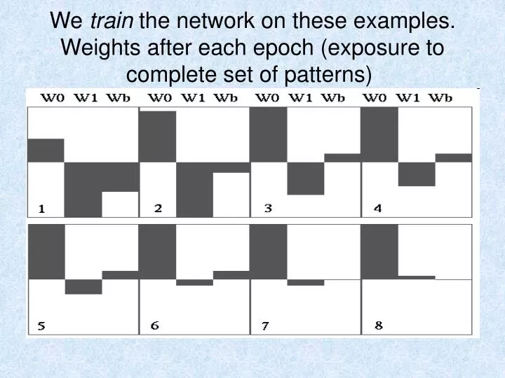
We train the network on these examples. Weights after each epoch (exposure to complete set of patterns) . At this point (8) the network has finished learning. Since (D-Y)=0 for all patterns, the weights cease adapting. Single perceptrons are limited in what they can learn:

E N D
We train the network on these examples. Weights after each epoch (exposure to complete set of patterns)
At this point (8) the network has finished learning. Since (D-Y)=0 for all patterns, the weights cease adapting. • Single perceptrons are limited in what they can learn: • If we have two inputs, the decision surface is a line. ... and its equation is I1 = (W0/W1).I0 + (Wb/W1)
Pattern Recognition - an example • Pattern recognition can be implemented by using a feed-forward
The network is trained to recognise the patterns T and H. The associated patterns are all black and all white respectively as shown below.
If we represent black squares with 0 and white squares with 1 then the truth tables for the 3 neurones after generalisation are; Top neuron
From the tables it can be seen the following associasions can be extracted: Here also, it is obvious that the output should be all whites since the input pattern is almost the same as the 'H' pattern. In this case, it is obvious that the output should be all blacks since the input pattern is almost the same as the 'T' pattern. Here, the top row is 2 errors away from the a T and 3 from an H. So the top output is black. The middle row is 1 error away from both T and H so the output is random. The bottom row is 1 error away from T and 2 away from H. Therefore the output is black. The total output of the network is still in favour of the T shape.
Back-Propagated Delta Rule Networks (BP) (sometimes known and multi-layer perceptrons (MLPs)) and • Radial Basis Function Networks (RBF) Are both well-known developments of the Delta rule for single layer networks. Both can learn arbitrary mappings or classifications. Further, the inputs (and outputs) can have real values
Back-Propagated Delta Rule Networks (BP) • is a development from the simple Delta rule in which extra hidden layers (layers additional to the input and output layers, not connected externally) are added. The network topology is constrained to be feedforward: i.e. loop-free - generally connections are allowed from the input layer to the first (and possibly only) hidden layer; from the first hidden layer to the second,..., and from the last hidden layer to the output layer.
The hidden layer learns to recode (or to provide a representation for) the inputs. More than one hidden layer can be used. • The architecture is more powerful than single-layer networks: it can be shown that any mapping can be learned, given two hidden layers (of units). • The units are a little more complex than those in the original perceptron
their input/output graph is • As a function: Y = 1 / (1+ exp(-k.(Σ Win * Xin)) • The graph shows the output for k=0.5, 1, and 10, as the activation varies from -10 to 10. • Training BP Networks • The weight change rule is a development of the perceptron learning rule. Weights are changed by an amount proportional to the error at that unit times the output of the unit feeding into the weight.
Running the network consists of • Forward pass: • the outputs are calculated and the error at the output units calculated. • Backward pass: • The output unit error is used to alter weights on the output units. Then the error at the hidden nodes is calculated (by back-propagating the error at the output units through the weights), and the weights on the hidden nodes altered using these values. • For each data pair to be learned a forward pass and backwards pass is performed. This is repeated over and over again until the error is at a low enough level (or we give up).
Radial basis function networks are also feedforward, but have only one hidden layer. Typical RBF architecture:
Like BP, RBF nets can learn arbitrary mappings: the primary difference is in the hidden layer.
RBF hidden layer units have a receptive field which has a centre: that is, a particular input value at which they have a maximal output. Their output tails off as the input moves away from this point.
Generally, the hidden unit function is a Gaussian: Gaussians with three different standard deviations.
Training RBF Networks. RBF networks are trained by • deciding on how many hidden units there should be • deciding on their centres and the sharpnesses (standard deviation) of their Gaussians • training up the output layer. • Generally, the centres and SDs are decided on first by examining the vectors in the training data. The output layer weights are then trained using the Delta rule. BP is
Unsupervised networks: • Simple Perceptrons, BP, and RBF networks need a teacher to tell the network what the desired output should be. These are supervised networks. In an unsupervised net, the network adapts purely in response to its inputs. Such networks can learn to pick out structure in their input. Paradigms of unsupervised learning are Hebbian lerning and competitive learning. Unsupervised learning is performed on-line • Paradigms of supervised learning include error-correction learning, reinforcement learning and stochastic learning. Usually, supervised learning is performed off-line
Transfer Function • The behaviour of an ANN (Artificial Neural Network) depends on both the weights and the input-output function (transfer function) that is specified for the units. This function typically falls into one of three categories: • linear (or ramp) • threshold • sigmoid
For linear units, the output activity is proportional to the total weighted output. • For threshold units, the output is set at one of two levels, depending on whether the total input is greater than or less than some threshold value. • For sigmoid units, the output varies continuously but not linearly as the input changes. Sigmoid units bear a greater resemblance to real neurones than do linear or threshold units, but all three must be considered rough approximations.
To make a neural network that performs some specific task, we must choose how the units are connected to one another, and we must set the weights on the connections appropriately. • The connections determine whether it is possible for one unit to influence another. The weights specify the strength of the influence.
We can teach a three-layer network to perform a particular task by using the following procedure: • We present the network with training examples, which consist of a pattern of activities for the input units together with the desired pattern of activities for the output units. • We determine how closely the actual output of the network matches the desired output. • We change the weight of each connection so that the network produces a better approximation of the desired output.
An Example to illustrate the teaching procedure in the previous slide • Assume that we want a network to recognise hand-written digits. We might use an array of, say, 256 sensors, each recording the presence or absence of ink in a small area of a single digit. The network would therefore need 256 input units (one for each sensor), 10 output units (one for each kind of digit) and a number of hidden units. • For each kind of digit recorded by the sensors, the network should produce high activity in the appropriate output unit and low activity in the other output units. • To train the network, we present an image of a digit and compare the actual activity of the 10 output units with the desired activity. We then calculate the error, which is defined as the square of the difference between the actual and the desired activities. Next we change the weight of each connection so as to reduce the error. We repeat this training process for many different images of each different images of each kind of digit until the network classifies every image correctly. • To implement this procedure we need to calculate the error derivative for the weight (EW) in order to change the weight by an amount that is proportional to the rate at which the error changes as the weight is changed. One way to calculate the EW is to perturb a weight slightly and observe how the error changes. But that method is inefficient because it requires a separate perturbation for each of the many weights. • Another way to calculate the EW is to use the Back-propagation algorithm, which has nowadays become one of the most important tools for training neural networks. It was developed independently by two teams, one (Fogelman-Soulie, Gallinari and Le Cun) in France, the other (Rumelhart, Hinton and Williams) in U.S.
The Back-Propagation Algorithm • In order to train a neural network to perform some task, we must adjust the weights of each unit in such a way that the error between the desired output and the actual output is reduced. This process requires that the neural network compute the error derivative of the weights (EW). In other words, it must calculate how the error changes as each weight is increased or decreased slightly. The back propagation algorithm is the most widely used method for determining the EW. • The back-propagation algorithm is easiest to understand if all the units in the network are linear. The algorithm computes each EW by first computing the EA, the rate at which the error changes as the activity level of a unit is changed. For output units, the EA is simply the difference between the actual and the desired output. To compute the EA for a hidden unit in the layer just before the output layer, we first identify all the weights between that hidden unit and the output units to which it is connected. We then multiply those weights by the EAs of those output units and add the products. This sum equals the EA for the chosen hidden unit. After calculating all the EAs in the hidden layer just before the output layer, we can compute in like fashion the EAs for other layers, moving from layer to layer in a direction opposite to the way activities propagate through the network. This is what gives back propagation its name. Once the EA has been computed for a unit, it is straight forward to compute the EW for each incoming connection of the unit. The EW is the product of the EA and the activity through the incoming connection.
Applications of neural networks • Modelling and Diagnosing the Cardiovascular System • Electronic noses • Marketing • Credit Evaluation • Targeted advertising • Face recognition • Facial expression recognition