Download
1 / 106
1.07k likes | 1.08k Views
Statistical Shape Modelling. Multimodal Interaction Dr. Mike Spann m.spann@bham.ac.uk http://www.eee.bham.ac.uk/spannm. Contents . Introduction Point distribution models Principal component analysis Shape modelling using PCA Case study. Face image analysis Model-based object location.

E N D
Statistical Shape Modelling Multimodal Interaction Dr. Mike Spann m.spann@bham.ac.uk http://www.eee.bham.ac.uk/spannm
Contents • Introduction • Point distribution models • Principal component analysis • Shape modelling using PCA • Case study. Face image analysis • Model-based object location
Introduction • Statistical shape models attempt to model the shapes of objects found in images • The images can either be 2D or 3D • Why ‘statistical’? • We normally attempt to build a ‘model’ of a shape from a training set of ‘typical’ shapes • Our model characterizes the variation of shapes within the training set • This variation is described by statistical parameters (eg. deviation from the mean shape)
Introduction • In the images of a hand, we want to represent the shape of each hand efficiently to enable us to describe the subtle variations in the shape of each hand • How? • Outline contour? • Not that easy to fit and we still have the problem of accurately determining contour descriptors such as B-spline parameters • Landmarks? • We have a fighting chance of finding suitable landmark points and we can describe discrete points using point distribution models
Introduction • We can apply this concept of shape representation using landmarks to face images • Significant facial features such as the lips, nose, eyebrows and eyes constitute the ‘shape’ of the face • As we will see, by modelling the spatial distribution of these landmarks across a training set, our model parameters will allow us to develop face and lip tracking algorithms
Introduction Landmarked face ‘Shape’
Introduction • So what do we mean by ‘shape’? • Shape is an intrinsic property of an object • Shape is not dependant on the position, size or orientation of the object • This presents us with a problem as we have to ‘subtract out’ these properties from the object before we determine its shape • In a training image database, it means we have to align the objects with respect to position, size and orientation before constructing our shape model • This process is normally done after landmark points have been extracted so we align the pointsets
Introduction rotate scale
Introduction • Why do we need a shape model? • A shape model is a global constraint on an objects shape • More effective than local constraints such as imposed by snake type algorithms • Essentially we are looking for a shape in a certain eigenspace (see later) in our search/tracking algorithm • What’s it got to do with multi-modal interaction? • In a speech recognition system, an effective approach is to combine the shape of the lips with audio descriptors • We need a real time lip tracking algorithm • Statistical shape model parameters can be feature descriptors • In general, facial feature tracking has many applications in areas such as biometric identification and digital animation
Point distribution models • We have seen how the boundary shape of an object can be represented by a discrete set of coordinates of ‘landmark points’ • Consider set of training images in a database, for example face images or hand images • Each image will generate a set of landmark points • A point distribution model (pdm) is a model representing the distribution of landmark points across the training images • It uses a statistical technique known as Principle Component Analysis (PCA)
Point distribution models ‘Shape’ Landmarked face
Point distribution models • We can label each point set xs for each training shape s=1..S • Our ultimate goal is to build a statistical model from our point sets • But until our point sets are aligned, any statistical model would be meaningless • We can imagine each xs to be a point in some 2n dimensional space (assuming there are n landmark points)
Point distribution models • We can superimpose our landmarks on a single image frame
Point distribution models • We can rotate/scale our images so they are registered
Point distribution models • Alignment of landmark points essentially registers the points by rotating/scaling to a common axis • It forms tight clusters of points in our 2n dimensional space for similarly shaped objects in the training set • As we shall see later, it then allows us to apply principal components analysis on these clusters • The idea is to try and describe the point distribution efficiently and represent the principal features of the distribution and hence the object shape
Point distribution models Aligned Unaligned
Point distribution models • How do we align our pointsets? • Let’s assume we have 2 pointsets • We are looking for a transformation T which when applied to xs aligns it with x's • We are looking for the transformation which minimizes E the sum of squared distances between the pointsets
Point distribution models • We can consider different types of transformation • Translation • Scaling • Rotation
Point distribution models • The rotation matrix is a simple axis rotation in 2D
Point distribution models • Rotation is an example of a similarity transform • The Euclidean length of the vectors is unchanged after such a transform • The general form of a similarity transform is : • The affine transform is an unrestricted transform and can include geometrical transforms which skew the (x,y) axes
Point distribution models • We will look at finding the optimum affine transformation which best aligns to pointsets • Thus we wish to find the parameters (a,b,c,d,tx,ty) which minimizes : • This is a straightforward but tedious exercise in calculus which is solved by differentiating the above equation with respect to the parameters (a,b,c,d,tx,ty)
Point distribution models • The result is expressed in terms of the following moments of the (x,y) coordinates of pointsets xs and xs’
Point distribution models • Note that (Sx,Sy)is the centre of gravity of pointset xs
Point distribution models • To simplify the algebra, let’s assume that the pointset xs is defined so that it is centred on the origin • This involves simply subtracting (Sx,Sy) from each landmark coordinate • This results in (Sx,Sy) =(0,0) which in turn leads to : • The final result for the rest of the parameters becomes :
Point distribution models • We can easily apply these equations to align two shapes expressed by the two pointsets xs and xs’ • A trickier problems is to align a set of pointsets {xs : s=1..S }in a training database • An analytic solution to the alignment of a set of shapes does exist • These techniques align each shape so that the sum of distances to the mean shape D is minimized :
Point distribution models • However, a simple iterative algorithm works just as well • Translate each pointset to centre at the origin • Choose an arbitrary pointset (eg s=0) as an initial estimate of the mean shape and scale each pointset to an arbitrary size (eg all |xs|=1) • Align all the pointsets with the current mean estimate using the affine transformation • Re-estimate the mean pointset from the aligned pointsets • Re-align the mean pointset with x0and re-scale to modulus 1 • If not converged go back to 3
Point distribution models • Step 5 is important in making the procedure well defined • Otherwise, the mean pointset is defined by the aligned point sets and the aligned pointsets are defined by the mean pointset • Convergence is usually determined when the estimated mean doesn’t change above some specified threshold • Typically convergence is in a couple of iterations
Principal component analysis • Principal component analysis (PCA) is an important statistical technique for analysing data and is crucial in understanding statistical shape models • PCA involves discovering patterns in data and what aspect of our data is important and what is less important • In particular, our data is multidimensional (eg pointsets) so PCA asks the question what dimensions are important (in other words account for significant variation in shape) and which are less important
Principal component analysis • PCA is analysing multidimensional data, in other words, random vectors • A random vector is a vector with random components • For example, n-component column vector xs • It is sometimes helpful to imagine xs being a random position in n-dimensional space and a set of these random vectors being a cloud of these points in this space
Principal component analysis • PCA attempts to determine the principal directions of variation of the data within this cloud Significant variation in this direction But not in this direction
Principal component analysis • We will review some basic measures of random vectors before introducing PCA • Mean vector • Covariance matrix
Principal component analysis • The covariance matrix is a sum of outer vector products and results in an nxn matrix • For example in the 2D case: • The covariance matrix is a 2x2 matrix with the diagonal elements being the data variance in each dimension • Essentially the covariance matrix expresses the variation about the mean in each dimension
Principal component analysis Variation in x expressed by σx Variation in y expressed by σy Un-correlated data Correlated data
Principal component analysis • A particularly popular is the Gaussian model where all of the statistical properties of the data are specified by the mean vector and covariance matrix • The probability distribution completely defines the statistics of the data • The exponent is a quadratic form which defines an ellipsoid in n-dimensional space which are the surfaces of constant probability
Principal component analysis Covariance matrix defines the ellipsoid axes
Principal component analysis • For correlated data the ellipsoids are oriented at some angle with respect to the axes • We are looking to determine the variations along each axis • If our data was uncorrelated, this variation would be the diagonal elements of the covariance matrix • Thus our goal is to de-correlate the data • Or, diagonalize the covariance matrix • This re-orients the ellipsoid to have its axes along the data coordinate axes • This is the goal of PCA • To determine the principal axes of the data which are the directions of the re-oriented axes
Principal component analysis Un-correlated data Correlated data
Principal component analysis • We will derive the equations of principal component analysis using simple linear (matrix-vector) algebra • Our data x are statistical features (in our example landmark pointsets) represented by a vector • PCA determines a linear transformation M of the data which diagonalizes the covariance matrix of the transformed data • Our transformed data is represented by vector b
Principal component analysis • It is fairly simple matrix algebra to determine the mean and covariance of the transformed vector y
Principal component analysis • We restrict ourselves to orthogonal transformation matrices • In other words, the columns of the matrix are orthonormal vectors • For the ithand jthcolumn vectors of M • We can then write
Principal component analysis • We are seeking Cb to be a diagonal matrix • This makes the previous equation an eigenvector/eigenvalue equation • Given an n x n matrix A, e is an eigenvector of A with associated eigenvalue λ where : • For an n x n (non-singular) matrix, there are n eigenvectors and eigenvalues • For a symmetric matrix (which the covariance matrix is), the eigenvectors are orthogonal • In other words, for 2 eigenvectors eiand ej
Principal component analysis • Let Фbe a matrix whose columns are the eigenvectors of the covariance matrix Cx • From the first equation • Let : • We then obtain
Principal component analysis • Because Фis a matrix whose columns are the eigenvectors of the covariance matrix Cx : • The λ’s are the eigenvalues of Cx • Finally, from the previous equation, since Фis an orthogonal matrix :
Principal component analysis • We can summarise our procedure so far • Given a random data vector x with covariance matrix Cx • We apply a transformation to the data which diagonalizes the covariance matrix • Фis a matrix whose columns are the eigenvectors of the covariance matrix Cx • The covariance matrix of b is now a diagonal matrix with diagonal elements being the eigenvalues of Cx