Download
1 / 9
90 likes | 326 Views
USA Income Distribution counter-business-cyclical trend Estimating Lorenz curve using continuous L 1 norm estimation Bijan Bidabad bijan_bidabad@msn.com . Lorenz curve. Skewness of income distribution. Functional form. Data. Estimation. Continuous L 1 norm smoothing. Gupta (1984)

E N D
USA Income Distributioncounter-business-cyclical trendEstimating Lorenz curve usingcontinuous L1 norm estimationBijan Bidabadbijan_bidabad@msn.com
Lorenz curve Skewness of income distribution Functional form Data Estimation Continuous L1 norm smoothing Gupta (1984) Bidabad (1989) µ , σ, med, kurtosis, skewness …
Continuous L1 norm smoothing Min: S = ||u||1 = ||y(x)-f(x,β)||1 β =∫xεI |y(x)-f(x,β)|dx Linear 1 parameter: Min: S = ∫xεI |y(x)-βx|dx β = ∫xεI |x||y(x)/x – β|dx y(x)/x < β if x < t y(x)/x = β if x = t y(x)/x > β if x > t Min: S = -∫0t |x|(y(x)/x-β)dx β,t +∫t1 |x|(y(x)/x-β)dx
Continuous L1 norm smoothing After equating partial derivatives of S respect to β and t to zero: y(√2/2) t = √2/2 β = ───── √2/2 Generalization to 2 parameters Min: S=∫xεI |y(x)-α-βx|dx α,β Solution: t1=1/4 t2=3/4 β = 2[y(3/4)-y(1/4) α = y(3/4)-(3/4)β = y(1/4)-(1/4)β
Lorenz curve (P(V|V≤v) , E(V|V≤v)/E(V)) ≡ ∫-∞v wf(w)dw (∫-∞v f(w)dw , ──────────) ≡ ∫-∞+∞wf(w)dw (x(v) , y(x(v))) Gupta (1984) y=xAx-1eu A>1 Bidabad (1989) y=xBAx-1eu A≥1 B≥1 x(v)= ∫0v f(w)dw y(x(v))= 1/E(w)∫0v wf(w)dw
Lorenz curve Gupta y=xAx-1eu A>1 min: ∫01 |ln y(x) - ln x - (x-1)ln A|dx A 1-√2/2 A = [−−−−]√2 x(v)=∫0v f(w)dw =1-√2/2 y(1-√2/2) Bidabad y=xBAx-1eu A≥1 B≥1 min: ∫01|x-1| |[lny(x)]/(x-1)-(lnx)/(x-1)-lnA|dx A,B B =-0.848ln[y(0.075)]+ 1.317ln[y(0.404)] A = [y(0.075)]1.289[y(0.404)]-3.681 x(v)=∫0v f(w)dw =0.075 x(v)=∫0v f(w)dw =0.404
Income distribution in USA Log-Normal Distribution
Thank youBijan Bidabadbijan_bidabad@msn.comhttp://www.geocities.com/bijan_bidabad/