Download
1 / 21
220 likes | 447 Views
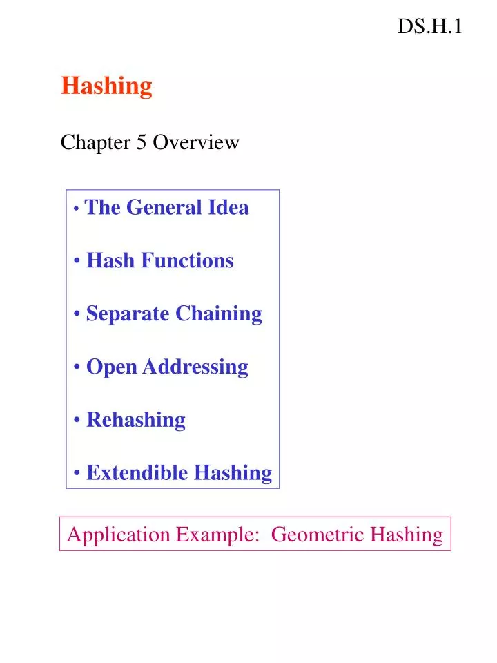
DS.H.1. Hashing. Chapter 5 Overview. The General Idea Hash Functions Separate Chaining Open Addressing Rehashing Extendible Hashing. Application Example: Geometric Hashing. DS.H.2. Why should we consider another indexing technique when B-trees are so great?.

E N D
DS.H.1 Hashing Chapter 5 Overview • The General Idea • Hash Functions • Separate Chaining • Open Addressing • Rehashing • Extendible Hashing Application Example: Geometric Hashing
DS.H.2 Why should we consider another indexing technique when B-trees are so great? • To avoid the multi-level index structure • on disk. • To get a small constant search time for • equality queries to databases. • To provide another structure that is useful • for internal memory look-up tables.
DS.H.3 HASHING Given: 1. a relatively large block of storage called the hash table 2. an attribute or key Possible Goals: 1. Insert: store the key and its value in the table. 2. Find: find the key in the table and return its value. 3. Delete: remove the key and its value from the table.
DS.H.4 Hash Function: A hash function maps keys to ‘random’ addresses within the hash table. Example: Let the hash table be N locations long. Suppose the keys are integers or can somehow be converted to integers. f(key) = key % N /* key modulo N */ is the most common, simple hash function. NOTE: in hashing, the potential number of possible keys is much greater than the number of keys in use at any given time.
DS.H.5 Example: Let N = 50 and suppose there are 300 possible keys, but we don’t expect to have more than 50 in the table at once. f(key) = key % 50 Key Table Address 1 1 49 49 256 6 75 25 125 25 175 25 collision There are many different ways to resolve collisions.
DS.H.6 First, a few more hash functions Numeric Keys: h1(key) = key % N h2(key) = extract(P, Q, key*C) /* Start at bit position P of key*C and extract Q bits to generate addresses in the correct range */ h3(key) = irand(N, key) /* Feed the key as a seed to a random number generator and normalize to an integer between 0 and N-1 */
DS.H.7 Character String Keys: h4(key) = char_sum(key) % N /* Add together the byte representations of each of the characters and normalize to table size */ h5(key) = extract(P, Q, char_product(key)) /* Multiply together the byte representations of each of the characters and extract Q bits starting at bit P to generate addresses in the correct range */ h6(key) = key[keysize – i –1] * 32 modulo table size (book’s Fig 5.5 is wrong) keysize - 1 i i = 0
DS.H.8 Separate Chaining Separate chaining is a collision strategy that uses linked lists to solve the collision problem. A “bin” of the hash table merely points to a linked list that hold all keys that hash to that bin. Bin 25 holds 3 different keys. 75 125 175 25 Separate chaining is very flexible, makes insertion and deletion easy, but it requires pointers, which isn’t so good on disk.
DS.H.9 Open Addressing Open addressing uses one big contiguous hash table. When there is a collision, it tries alternate locations, using the function: hi(x) = ( hash(x) + F(i) ) % N It first tries h0(x), then h1(x), etc. until it finds the key in the table or comes to an empty cell to put it in. 75 125 175 h0(x) = 25 So how do we define F(i)? h1(x) = 30 h2(x) = 35
DS.H.10 • There are several common ways: • Linear Probing • /* F(i) is a linear function of i */ • F(i) = i is most common. • It tries the next position for each probe. • h(0) = hash(x) • h(1) = hash(x) + 1 • h(2) = hash(x) + 2 • This is simple, but has the problem of • primary clustering. • Clusters develop in the table and most • keys lead to some search.
DS.H.11 2. Quadratic Probing /* F(i) is a quadratic function of i */ F(i) = i This spreads out the probes more. h(0) = hash(x) h(1) = hash(x) + 1 h(2) = hash(x) + 4 This works better, but some secondary clustering effects have been reported. 2 Theorem: If quadratic probing is used and the table size is prime, then a new element can always be inserted if the table is at least half empty. (proof by contradiction is readable)
DS.H.12 3. Double hashing /* Use a second hash function */ F(i) = i * hash2(x) This spreads out the probes more. h(0) = hash(x) h(1) = hash(x) + 1 * hash2(x) h(2) = hash(x) + 2 * hash2(x) Variant: use a sequence of hash functions h(i) = x % N i+1 Disadvantage of Open Addressing: deletion is difficult. Why?
DS.H.13 Rehashing /* If the table is getting too full, rebuild it with twice the space. Do this infrequently and at night. */ 0 1 2 3 4 5 6 7 8 9 70 Louis Smith 52 Kate Green 94 Craig Mir 45 John Smith 97 Ray Finch 0 1 2 3 4 70 Louis Smith 45 John Smith 52 Kate Green 97 Ray Finch 94 Craig Mir Why is 45 in bin 1 when 45 % 5 = 0?
DS.H.14 Complexity Analysis Let N be the number of entries in the table at the current time. Let T be the table size. Let = N/T be the load factor. • Chaining: • N can be larger or smaller than T. • e.g. We can have 10 lists of 5 elements each. • 1. What is the longest any list can be? • 2. What is the shortest any list can be? • 3. What is the average length of a list?
DS.H.15 Complexity Analysis N entries, table size T, =N/T • Chaining: • 1. What is the longest any list can be? N • 2. What is the shortest any list can be? 0 • What is the average length of a list? • When =1, N = T, so average 1 element / list. • When =2, N = 2T, so average 2 elements / list. • General case: the average list has elements. Search time:T(N,T) = c1 + c2(/2) = O() = O(N/T) hash search a list Insertion time: O(1) why?
DS.H.16 Open Addressing: N T, << 1 (full is BAD) Linear Probing: What is the average number of cells probed in a successful search? = percentage of full cells. (1- ) is the percentage of empty cells. 1/(1- ) is the number of cells searched before an empty one is found. Maximum probes is 1 + 1/(1- ) . Average probes is ½(1 + 1/(1- ) ) .
DS.H.17 Linear Probing: = N/T = percentage of full cells. Successful Search: ½(1 + 1/(1- ) ) Insert or Unsuccessful Search: ½(1 + 1/(1- ) ) • Examples: • = .25 1 • = .99 50 Examples: = .1 1 = .5 3 = .75 9 = .99 5000
DS.H.18 Extendible Hashing Extendible hashing is a fast access method for dynamic files. For data on disk, we don’t want to chase pointers. Suppose that m (key, data) pairs fit in one disk block and that the hash function returns a bit string. • Keep a directory that is organized according • to the leading D bits of the hash value. • D changes dynamically as the table grows. • - Use only enough bits to distinguish blocks.
DS.H.19 D=1 (bit) 0 1 0 0 0 0 0 0 1 0 0 1 0 0 0 1 0 1 1 0 0 0 1 0 0 1 1 0 1 0 1 1 0 0 1 0 Suppose we add key 0010. It belongs in bucket 0, which is full. So we split it into buckets 00 and 01. 0 0 0 1 1 0 1 1 D=2 1 00 01 00 0 0 00 1 0 01 0 0 0 1 0 1 011 0 1 0 0 0 1 0 0 1 1 0 1 0 1 1 0 0
DS.H.20 In extendible hashing, the index grows as needed. Complexity: N: entries M: block size Expected number of leaves: (N/M) log e Expected directory size: O(N / M) The bigger M is the better. 2 1+1/M
DS.H.21 Hashing Applications • in compilers: to store and access identifiers • in databases: for fast equality queries • in image analysis for storing large structures • Region Adjacency Graph Construction • Geometric Hashing Large number of regions with only a small percentage active at one time. Large number of (object, transform) pairs requiring lots of quick lookups.