Sensor Range Analysis

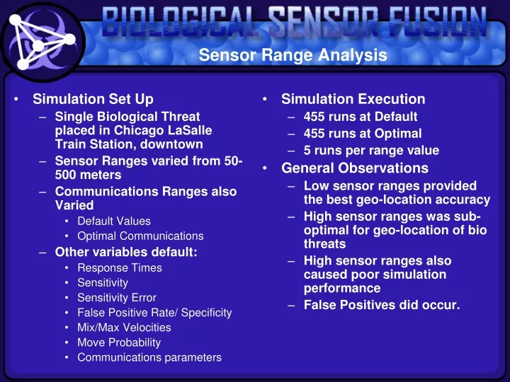
1. Sensor Range Analysis Simulation Set Up Single Biological Threat placed in Chicago LaSalle Train Station, downtown Sensor Ranges varied from 50-500 meters Communications Ranges also Varied Default Values Optimal Communications Other variables default: Response Times Sensitivity Sensitivity Error False Positive Rate/ Specificity Mix/Max Velocities Move Probability Communications parameters Simulation Execution 455 runs at Default 455 runs at Optimal 5 runs per range value General Observations Low sensor ranges provided the best geo-location accuracy High sensor ranges was sub-optimal for geo-location of bio threats High sensor ranges also caused poor simulation performance False Positives did occur.

2. Typical Simulation Execution Run Epidemic-SI Communications Bio Threat release in Chicago LaSalle Train Station Low sensor range yields high Cordon accuracy

3. Range vs. Latency • Conclusions: • Except at sensor ranges <150meters, sensor range has almost no impact on latency • Most of the variance observed here is due to sub-optimal communications

4. Range vs. Latency (cont.) • Conclusions: • Here is the same latency range analysis using optimal communications • Worst case latency is reduced by 50% • Variance is much decreased for sensor ranges >150m and latency is typically 3 minutes or less

5. Range vs. Hop Count • Conclusions: • Sensor Range has no impact on Hop Count. This is driven solely by communications range. • The variance seen here is from sub-optimal communications range settings.

6. Range vs. Hop Count (cont.) • Conclusions: • Here is analysis again with optimal communications ranges. Note hop count (when optimized) is almost always six degrees of separation or less: “Small World Communication”

7. Range vs. Neighbors • Conclusions: • Sensor Range also has no impact on Neighbor Quantity.

8. Range vs. Neighbors (cont.) • Conclusions: • With optimal Communication Ranges used, neighbors range from 0 to 27 – i.e. still a high level of network disconnection.

9. Range vs. Power Remaining • Conclusions: • With less than optimal communications, the impact of Sensor Range on Power is difficult to determine. Values vary widely.

10. Range vs. Power Remaining (cont.) • Conclusions: • With optimal communications, its easy to see that Sensor Range does have a slight impact on remaining power, but only at ranges <100meters.

11. Range vs. Coverage • Conclusions: • As expected, overall city sensor Coverage increases logarithmically as sensor range increases. • Variance is much better at low ranges, and for optimal sensor ranges, typically 30% or less • Since Communications Range has no impact on Coverage, the default and optimal run results were exactly the same.

12. Analysis Conclusions • Sensor Range • Sensor Range has only a slight impact on latency and remaining power for ranges <100m. • Coverage increases logarithmically with sensor range. • Sensor Range has no impact on hop count or neighbors. • Sensor Ranges >150m provide little or no benefit for Biological Sensor Fusion • Other Inferences • Low sensor ranges provided the best geo-location accuracy • With both optimal communications and sensor ranges • A fused DHS Operations Center result is reasonable in under 5 minutes after biological agent release • Less than 10% of average Tier III power is needed • The network represents “Small World Communication” • These conclusions are based on the chosen 276 sensors deployed in Chicago District 001.