Quantification of Habitat for Snag-dwelling Invertebrates: Incorporation into a Dynamic Model.

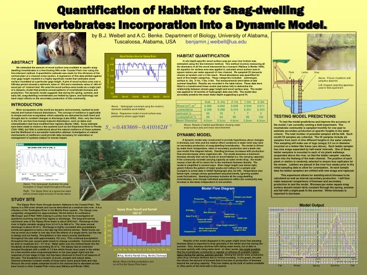
1. Quantification of Habitat for Snag-dwelling Invertebrates: Incorporation into a Dynamic Model. by B.J. Weibell and A.C. Benke. Department of Biology, University of Alabama, Tuscaloosa, Alabama, USA benjamin.j.weibell@ua.edu HABITAT QUANTIFICATION In situ depth-specific wood surface area per area river bottom was estimated using the line-intersect method. This method involves measuring all the diameters of all the wood intersected by a transect (Wallace & Benke 1984). An equation for surface area was applied to calculate wood surface area in square meters per meter squared of river channel. We sampled 25 transects chosen at random over a 3 km reach. Wood abundance was quantified for each of five height categories. These categories included: submerged, surface to .5m, .5-1m, 1-2m, 2-3m. The measurements were taken at late summer baseflow. Results are recorded in the table below. These data were fitted to a transformed linear model (see below left) to determine the relationship between stream gage height and wood surface area. The model was applied to 18 months of hydrograph data (see left). The model also accurately predicts the mean water depth suggesting a good fit. ABSTRACT We estimated the amount of wood surface area available to aquatic snag-dwelling invertebrates in a free-flowing fifth-order Coastal Plain river using the line-intersect method. A quantitative estimate was made for five divisions of the vertical plain of a channel cross section. A regression of this data plotted against river gage height resulted in a highly significant model that estimates wood surface inundated at a particular gage height. A plot of wood surface area over a 548-day period showed a minimum value of .304 and a maximum value of .465 m2 wood per m2 channel bed. We used the wood surface-area model as a major part of a dynamic model that predicts annual patterns of invertebrate biomass and production. The dynamic model suggests that during the spring, summer, and early fall, snag-dwelling invertebrates are limited by space, and hydrology can have major effects on the secondary production of this community. INTRODUCTION River ecosystems of the world are dynamic environments, marked by both natural and human-induced disturbance. The concept of resilience is applicable to stream and river ecosystems which naturally are disturbed by both flood and drought due to constant changes in discharge (Lake 2000). Also, very few rivers in the U.S. are free from human-induced disturbance, such as dams and channelization that have modified flow regimes (Benke 1990). Some attempts have been made to restore a few systems such as the Kissimmee River in Florida (Toth 1998), but little is understood about the natural resilience of these systems and the likelihood of a successful restoration attempt. Investigation of natural mechanisms of resilience could provide data necessary for restoration or management of systems subject to human impact. STUDY SITE The Sipsey River flows through western Alabama in the Coastal Plain. The Sipsey is a fifth-order stream and can be described as a medium-size river. It is a tributary of the Tombigbee River in the Mobile River system. The Sipsey runs completely unregulated for approximately 184 km before its confluence (McGregor and O’Neil 1992) making it a prime river for the investigation of questions involving natural flow regime or discharge. The long and narrow catchment area of the Sipsey River basin is about 2043 km2. Discharge of this river is highly variable ranging from 2.5 m3/s to 566 m3/s. The mean annual discharge is about 25 m3/s. Discharge is highly correlated with precipitation events and appears to have a two-day lag time behind storms. Water levels can rise as much as a meter in one day from the effects of a single storm, but the rise is steady and not flashy. Precipitation in this area is evenly distributed throughout the year with approximately 142 cm/y. This continual precipitation throughout the year causes water levels to change constantly. Currents tend to be slow to moderate (0.2 – 0.7 m/s). Water spills over the channel bank into the floodplain at discharges exceeding 56 m3/s. The Sipsey has an extensive forested floodplain with a width of 1-3 km which floods most years in the winter for a few months when evapotranspiration is low (see graph right) and the response of river stage is high, but has been observed to flood in all seasons of the year. The floodplain is a mosaic of pools, sloughs and oxbow lakes. Channel substrate consists mostly of loose sand, some gravel beds and clay. Wood is the most stable substrate found in the channel and is abundant as has been found in other Coastal Plain rivers (see Wallace and Benke 1984). Above- Picture of platform with samplers attached Left- Diagram depicting apparatus used in field experiment Above- Hydrograph converted using the model to represent available wood habitat Below- Regression model of wood surface area predicted by stream gage height TESTING MODEL PREDICTIONS To test the model predictions and improve the accuracy of the model, I am currently running a field experiment. The invertebrate community is sampled monthly for one year to estimate secondary production at specific heights in the water column. The total number of potential samples will be 648. Each month 54 samples are collected. The 54 samples include six samples from each of nine different heights in the water column. This sampling will make use of logs (snags) 2-5 cm in diameter mounted on a ladder-like frame (see above). Each ladder sampler has nine snags separated by half-meter intervals. One of these ladder samplers is mounted to each of six plank walkways suspended above the river, so that the ladder sampler reaches down into the thalweg of the main channel. The position of each plank or station is randomly selected to ensure true replicates for the stream. Ladders are placed in the river four weeks prior to the initial sampling date to allow for colonization. At each sample date the ladder samplers are refitted with new snags and replaced. This experiment allows for standing-stock biomass to be calculated as well as interval secondary production. I will then make seasonal comparisons of biomass and secondary production to test the model. Biomass per meter square snag surface should remain fairly constant through the spring, summer and fall with a slight peak in the summer. Winter biomass is expected to decrease. Above- Results of habitat quantification showing mean wood surface area and mean wood diameter DYNAMIC MODEL A dynamic model was constructed to provide hypotheses about changes in biomass over time and the relative effect variations in water level may have on secondary production of snag-dwelling invertebrates. The model is driven by water level, temperature, rates of secondary production and a death rate (see model flow diagram below). Standing biomass increases with production flow and decreases when organisms die. The model assumes a maximum biomass density that can be found on wood habitat (i.e. the carrying capacity). If the community exceeds carrying capacity as water levels drop, the model causes a fast die-off to return the to the maximum biomass density. The model is simplified in several ways. River stage height (see below right, green) follows the pattern of major peaks and valleys for a sample year (compare to actual data in USGS Hydrograph plot, far left). Temperature (see below right, orange) shows generalized seasonal trends, ignoring smaller scale fluctuations. Standing biomass includes all the snag-dwelling invertebrates, even though individual populations within the community may increase or decrease independent of one another. Results of the model displayed in the graph (right) show that standing biomass (blue) is expected to drop generally in the winter and rise during the summer. Also, biomass declines with falling water levels, but is able to increase quickly with rising water level. In other words, the model predicts that the invertebrate community is capable of utilizing all available habitat space during the spring, summer and fall. During the winter when production rates drop, biomass declines due to normal mortality. In the graph, the pink line shows the amount of biomass that is lost due to production of biomass beyond the carrying capacity. This loss makes up the bulk of carbon available to other parts of the food web in this system. Above- This hydrograph illustrates the great fluctuation in stage height throughout the year. Right- The Sipsey River at a typical low-water period reveals large amounts of woody debris. Model Flow Diagram Model Output Above- Mean monthly precipitation and run-off for the Sipsey River basin Fall Winter Spring Summer Fall