Download

1 / 58
580 likes | 929 Views
Elasticity. IB-SL Economics Mr. Messere - CIA 4U7 Victoria Park S.S. Outline. I. Introduction II. Elasticity of Demand A. Definition B. Degrees of Elasticity of Demand C. Relationship between E d and Total Revenue D. Determinants of Elasticity of Demand

E N D
Elasticity IB-SL Economics Mr. Messere - CIA 4U7 Victoria Park S.S.
Outline I. Introduction II. Elasticity of Demand A. Definition B. Degrees of Elasticity of Demand C. Relationship between Ed and Total Revenue D. Determinants of Elasticity of Demand III. Other Elasticities A. Income Elasticity of Demand B. Cross Price Elasticity of Demand C. Elasticity of Supply D. Determinants of Elasticity of Supply
Coffee Question Consider the following: • An economist was called in to consult for a coffee shop that was losing money. • One manager thought they needed to raise prices in order to make more money on each coffee sold. • The other manager thought that lowering prices would make more money because a lot more coffee could be sold. Who was right?
Coffee Question • The answer is - it depends. On what? • If you lower the price - will the new sales offset the loss in revenue on each coffee? • If you raise your price - will the loss in sales be offset by the increase in price of coffee? • In other words, how much will the quantity demanded change when price changes?
Demand • We know, from the Law of Demand, that price and quantity demanded are inversely related. • Now, we are going to get more specific in defining that relationship • We want to know just how much will quantity demanded change when price changes? That is what elasticity of demand measures.
Elasticity of Demand • Elasticity of Demand (Ed) measures the responsiveness of the quantity demanded (Qd) of a good to a changein its price (P). Ed = % in Qd (Note that means “change”) % in P Ed = [(Q2-Q1)/Q1] ÷ [(P2-P1)/P1] • Also note that the law of demand implies Ed is negative. We will ignore the negative sign when discussing price elasticity of demand.
Calculating Elasticity of Demand • There are two methods for calculating elasticity - point and arc methods. • We will be examining the point method.
Point Elasticity P Consider the following Demand Curve: 6 5 2 D 1 0 Qd 2 3 6 7
Point Elasticity P A …and let’s say we want to find the Elasticity of Demand as we move from point A to Point B... 6 B 5 2 D 1 0 Qd 2 3 6 7
Point Elasticity • We know • Ed = % in QdorEd = [(Q2-Q1)/Q1] ÷ [(P2-P1)/P1] % in P • To calculate Ed from point A to B: • [(3-2)/2] [(5-6)/6] • 1/2 ÷ -1/6 • 3 (since negative sign ignored) • Calculate Ed from point C to D on the same curve
Point Elasticity P 6 5 C 2 D 1 0 Qd 2 3 7 8
Point Elasticity • Recall: • Ed = % in QdorEd = [(Q2-Q1)/Q1] ÷ [(P2-P1)/P1] % in P • To calculate Ed from point C to D: • [(8-7)/7] [(1-2)/2] • 1/7 ÷ -1/2 • 2/7 or 0.29 (since negative sign ignored)
Point Elasticity • Note that Ed is different at different places along the curve. • Specifically, it gets smaller as you move down the curve • Note that elasticity and slope are NOT the same thing. • One last calculation - let’s find the elasticity of demand going from point D to point C on the same curve
Point Elasticity • Recall: • Ed = % in Qdor Ed = [(Q2-Q1)/Q1] ÷ [(P2-P1)/P1] % in P • To calculate Ed from point D to C: • [(7-8)/8] [(2-1)/1] • -1/8 ÷ 1 • 1/8 or 0.13 (since negative sign ignored)
How Do We Interpret Elasticity? • The number we get from computing the elasticity is a percentage - there are no units. • We can read it as the percentage change in quantity for a 1% change in price
How Do We Interpret Elasticity? • Thus, if Ed = 2, that means on that part of the demand curve, a 1% change in price will cause a 2% change in quantity demanded. • Or if we extrapolate, a 10% change in price will cause a 20% change in quantity demanded, and so on.
Degrees of Demand Elasticity • Perfectly Inelastic Demand • Ed = % in Qd % in P • Ed = 0 % in P • Ed = 0 • No matter how much price changes, consumers purchase the same amount of the good. • Example: Insulin
P Qd Elasticity Perfectly Inelastic Demand ED = 0 0
Degrees of Ed • Inelastic Demand • Ed = % in Qd % in P • Ed < 1 (in absolute value) • % in Qd < % in P • For every 1% change in P, Qd changes by less than 1%
Elasticity Relatively Inelastic P 0 Qd
Degrees of Ed • Unitary Elastic Demand • Ed = % in Qd % in P • Ed = 1 (in absolute value) • % in Qd = % in P • For every 1% change in P, Qd changes by 1% (in opposite direction)
Unitary Elastic Demand P Unitary Elastic 0 QD
Degrees of Ed • Elastic Demand • Ed = % in Qd % in P • Ed > 1 (in absolute value) • % in Qd > % in P • For every 1% change in P, Qd changes by more than 1% (in opposite direction)
P Qd Elasticity Relatively Elastic 0
Degrees of Ed • Perfectly Elastic Demand • Ed = % in Qd % in P • Ed = % in Qd 0 • Ed = infinity • The price of the good never changes, no matter how much consumers purchase of the good.
Elasticity P Perfectly Elastic Demand ED = œ 0 Qd
Generalizing about Elasticity • Notice that the vertical (perfectly inelastic) demand curve has an elasticity of zero and the flat (perfectly elastic) demand curve has an elasticity of infinity. • As the demand curve goes from vertical to horizontal the elasticity is going from 0 to infinity • In other words, the flatter the demand curve, the greater the elasticity or if the curve becomes more vertical, then demand becomes more inelastic
The Coffee Problem • Back to the Coffeehouse question - should they raise or lower price? • We said that depended on how much sales will change when they change price • In other words, it depends on the elasticity
Total Revenue & Elasticity • Total Revenue = Price (p) x Quantity (q) • The coffeehouse is interested in how TR (total revenue) changes as p and q change
Total Revenue Calculation - Example • Price $1 Qd = 100 • TR = $100 • Price $3 Qd = 90 • TR = $270 • Price $4 Qd = 50 • TR = $200 • Price $5 Qd = 30 • TR = $150
P 10% TR DCoffee Qd Total Revenue and Elasticity • Let’s say demand is inelastic. Then if the coffeehouse raises prices 10%, the sales will drop by less than 10% • In other words, the gain in revenue from higher prices is greater than the loss in revenue from lost sales. Therefore, Total Revenue will rise
P Qd Total Revenue and Elasticity • If they lowered prices, though, the loss of revenue from higher prices would be greater than the gain from increased sales, so Total Revenue will fall 10% TR DCoffee
P 10% DCoffee TR Qd Total Revenue and Elasticity • Let’s say demand is elastic. Then if the coffeehouse raises prices 10%, the sales will drop by more than 10% • In other words, the gain in revenue from higher prices is less than the loss in revenue from lost sales. Therefore, Total Revenue will fall
Total Revenue and Elasticity • If they lowered prices, though, the loss of revenue from higher prices would be less than the gain in revenue from increased sales, so Total Revenue will rise P 10% DCoffee TR Qd
Total Revenue and Demand • So we can look at what happens to total revenue as we move down a demand curve • As we move down a demand curve we know that demand is elastic and as we lower price further demand becomes less elastic until we hit unit elasticity, at which point total revenue begins to fall and demand becomes more inelastic
Total Revenue and Demand ED = infinite $ Unitary Elastic Ed = 1 Elastic Ed >1 Inelastic Ed < 1 ED = 0 Q Ed = 1 $ Ed > 1 Ed < 1 Total Revenue Q
Total Revenue Test • If P and Total Revenue Move Together • Demand is Inelastic • If Qd and TR Move Together • Demand is Elastic • If changes in P or Qd Don’t Change TR • Demand is Unitary Elastic
Determinants of Ed Availability of Substitutes • As there are more substitutes, demand is more elastic • With fewer substitutes, demand is more inelastic • Example: • Coca-Cola has many substitutes and hence, demand is very elastic • Insulin has no substitutes for diabetic and hence, demand is very inelastic.
Determinants of Ed Percentage of Income Spent on Commodity • The less expensive a good is as a fraction of our total budget, the more inelastic the demand for the good is (and vice versa). • Example: • Price of cars go up 10% (from $20,000 to $22,000) • Price of toothpicks rise by 10% (from $2 to $2.20) • Demand is more (elastic) affected by the price of cars increasing vs. the increase in the price of toothpicks (price inelastic).
Determinants of Ed Time • The longer the time frame is, the more elastic the demand for a good is (and vice versa). • Example - Price of Gasoline Increases • Immediately: can’t do much, still need to get to work, school, etc. • Short-run: find a car pool, ride bike, public transit • Long-run: next car you buy uses less gas.
Determinants of Ed Nature of the Product - Necessities vs. Luxuries • The more necessary a good is, the more inelastic the demand for the good (and vice versa). • Example: Insulin
Income Elasticity of Demand • Income Elasticity of Demand (Ey) - measures the responsiveness of quantity demanded to changes in income (Y). • Ey = % in Qd % in Y • Ey = ( Q/Q) ÷ ( Y/Y) • Note that the negative sign is important!
Normal Goods • Typically, if our income rises, we buy more and vice versa. These types of goods are called normal goods. • EdY > 0 - normal good
Inferior Goods • There are some goods we buy less of as our income grows and more of as our income falls. • For instance, in university you’ll probably eat Macaroni & Cheese. But when you get a high paying job (as all V.P. grads do) you will probably buy less Mac and Cheese. • If a good’s elasticity is EdY < 0 it is an inferior good
Cross Price Elasticity of Demand • Another type of elasticity is the Cross Price Elasticity. This measures how changes in the price of one good can affect the quantity demanded of another • Cross Price Elasticity of Demand (EAPB) - measures the responsiveness of quantity demanded of good A when the price of good B changes.
Cross Price Elasticity of Demand • EAPB = % in Qd of Good A % in P of Good B EAPB = (QA / QA ) (PB / PB) • Note that the sign DOES matter for this elasticity also!
Substitute Goods • Consider Coke and Pepsi. If the price of Coke goes up, what would you expect to happen to the demand for Pepsi? • It will rise, since people will buy less Coke and more Pepsi. Thus the Demand for Pepsi will rise. • So the bottom of the elasticity fraction is positive and top of the elasticity fraction is positive.
Substitute Goods This relationship is called substitutes and can be seen when EA,B> 0.
Complement goods • Consider Washing Machines and Dryers. If the price of Washing Machines rises, what would you expect to happen to the demand for Dryers? • It will fall, since people will buy less washers at the new price, they will need less dryers. • So the bottom of the elasticity fraction is positive and top of the elasticity fraction is negative.