Download
1 / 66
680 likes | 699 Views
Neuromorphic Signal Processing for Auditory Scene Analysis. Jose C. Principe, Ph.D. Distinguished Professor and Director Computational NeuroEngineering Laboratory, University of Florida Gainesville, FL 32611 principe@cnel.ufl.edu http://www.cnel.ufl.edu. Table of Contents.

E N D
Neuromorphic Signal Processing for Auditory Scene Analysis Jose C. Principe, Ph.D. Distinguished Professor and Director Computational NeuroEngineering Laboratory, University of Florida Gainesville, FL 32611 principe@cnel.ufl.edu http://www.cnel.ufl.edu
Table of Contents • The need to go beyond traditional signal processing and linear modeling. • Examples: • Dynamic Vector Quantizers. • Signal to Symbol Translators • Entropy Based learning as a model for information processing in distributed systems.
DSP for Man-Made Signals • Digital Signal Processing methods have been developed assuming linear, time invariant systems and stationary Gaussian processes. • Complex exponentials are eigenvectors of linear systems • FFTs define frequency in an interval • Wiener filters are linear optimal for stationary random processes. • Markov models are context insensitive
Neurobiology reality • In order to become more productive we should develop a new systematic theory of biological information processing based on the known biological reality. • Decomposition in real exponentials (mesoscopic) • Local time descriptors (spike trains) • Nonlinear dynamical models • Adaptive distributed representations
Why delay a Neuromorphic Theory of Signal Processing? • A revamped framework is needed to understand biological information processing. It should be based on the distributed nature of the computation, the nonlinear nature of the dynamic PEs, the competition and association of the interactions at different space temporal scales. • Here we will be showing three examples of how the addition of dynamics have impacted conventional models and is helping us find new paradigms for computation.
Types of Memory • Generalized feedforward (gamma memory -- see Principe et al) • Spatial feedback
Temporal SOM Research • Basically two approaches for temporal self-organizing map (SOM): either memory is placed at the input (embedding) or at the output. See: • Kangas: external memory or hierarchical maps • Chappell and Taylor, Critchley: time-constant at each PE • Kohonen and Kangas: hypermap • Goppert and Rosenstiel: combined distance to input and distance to last winner
SOMs for Dynamic Modeling • Principe et al. applied temporal SOMs for local nonlinear dynamical modeling. • SOMs were used to cluster the NASA Langley supersonic wind tunnel dynamics. From the SOM weights, optimal filters were derived to predict the best control strategy to keep the tunnel at the optimum operating point.
SOMs for Dynamic Modeling • See also Ritter and Schulten.
Biological Motivation - NO • Nitric Oxide (NO) exists in the brain • NO produced by firing neurons • NO diffuses rapidly with long half-life • NO helps control the neuron’s synaptic strength (LTP/LTD) • NO is believed to be a “diffusive messenger” • Krekelberg has shown many interesting properties.
Biological Activity Diffusion • Turing’s Reaction-diffusion equation • Biological method of combining spatial (reaction) info with temporal info (diffusion) • R-D Equations can create wave-fronts • need excitable, nonlinear kinetics, and relaxation after excitation • Example Fitzhugh-Nagumo equations
Temporal Activity Diffusion-TAD • Goal is to create a truly distributed, spatio-temporal memory • Similar to NO diffusion in the SOM outputs • Activity “diffused” to neighboring PEs • lowers threshold of PEs with temporally active neighbors • creates temporal and spatial neighborhoods
SOM-TAD • Models diffusion with a traveling wave-front • Activity decays over time
SOM-TAD Equations • Exponential decay of activity at each PE • Activity creates traveling wave (build-up) • Winner selected including “enhancement” • Normal SOM update rule
SOM-TAD Memory • TAD creates a spatially distributed memory
SOM-TAD Application • Adjustable wave-front speed and width • Temporally self-organize spoken phonemes • words ‘suit’ and ‘small’ • Sampled at 16KHz, 3 bandpass filters (0.6-1.0 Khz, 1.0-3.5 KHz, and 3.5-7.4 KHz) • See also Ruwisch, et. al.
Phoneme Organization s Probabilities with TAD m a u t l Probabilities without TAD
Phoneme Organization Results Winners and Enhancement
Plasticity • Temporal information creates plasticity in the VQ Without temporal info With temporal info
Tessellation Dynamics This demonstration shows how the GasTAD uses the past of the signal to anticipate the future. Note that the network has FIXED coefficients. All the dynamics that are seen come from the input and the coupling given by the temporal diffusion memory mechanism. Run Demonstration
VQ Results VQ=[27,27,27,27,27,27,27,27,27,27,27,27,27,27] VQ=[12,12,16,16,25,25,25,25,27,27,27,27,27,27 GAS-TAD removes noise from signal using temporal information to “Anticipate” the next input
VQ for Speech Recognition • GAS-TAD used to VQ speech and remove noise using temporal information • 15 speakers saying the digits one through ten -- 10 training, 5 testing • Preprocessing: • 10 KHz sampling, 25.6 ms frames, 50% overlap • 12 liftered, cepstral coefficients • Mean filtered 3 at a time to reduce input vectors
Training • Each VQ trained with 10 instances of desired digit plus random vectors from other 9 digits
Recognition System • An MLP with a gamma memory for input was used for recognition • Winner-take-all determines digit
System Performance • Compare no VQ (use raw input), vs. NG VQ, vs. GAS-TAD VQ • GAS-TAD VQ reduces errors by 40% and 25% • HHM provided 81% (small data base)
Conclusions • TAD algorithm uses temporal plasticity induced by the diffusion of activity through time and space • Unique spatio-temporal memory • Dynamics that can help disambiguate the static spatial information with temporal information. Principe, J., Euliano N., Garani S., “Principles and Networks for self-organization in space time”, Special Issue on SOMs, Neural Networks, Aug 2002 (in Press).
New paradigms for computation • Interpretation of real world requires two basic steps: • Mapping signals into symbols • Processing symbols For optimality both have to be accomplished with as little error as possible.
New paradigms for computation • Turing machines process symbols perfectly But can they map signals-to-symbols (STS) optimally? • I submit that STS mappings should be implemented by processors that learn directly from the datausing non-convergent (chaotic) dynamics to fully utilize the time dimension for computation.
New paradigms for computation • STS processors interface the infinite complexity of the external world with the finite resources of conventional symbolic information processors. • Such STS processors exist in animal and human brains, and their principle of operation are now becoming known. • This translation is not easy if we observe the size of animal cortices…..
New paradigms for computation • Our aim (w/ Walter Freeman) is to construct a neuromorphic processor in analog VLSI that operates in accordance with the nonlinear (chaotic)neurodynamics of the cerebral cortex. • Besides hierarchical organization, nonlinear dynamics provides the only known mechanism that can communicate local effects over long spatial scales. Except that chaos does not need any extra hardware.
Freeman’s K0 model • Freeman’s modeled the hierarchical organization of neural assemblies using K - (Katchalsky) sets • The simplest (K0) is a distributed, nonlinear, two variable dynamic model
Freeman’s PE (KII) • The fundamental building block is a tetrad of K0 nodes interconnected with fixed weights The Freeman PE functions as an oscillator. Frequency is set by a,b and the strength of negative feedback.
Freeman’s KII model • An area of the cortex is modeled as a layer of Freeman PEs, where the excitatory connections are trainable. This is a set of coupled oscillators in a space-time lattice. adaptive adaptive
Freeman’s KII model • How does it work? PEs oscillate (characteristic frequency) when an input is applied, and the oscillation propagates. The space coupling depends on the learned weights, so information is coded in spatial amplitude of quasi-sinusoidal waves.
Channels 1 2 3 ..... 20 ..... Freeman’s KII model
Freeman’s KIII model • The olfactory system is a multilayer arrangement of Freeman PEs connected with dispersive delays and each layer with its natural (noncomensurate) frequencies. End result: the system state never settles, creating a chaotic attractor with “wings”.
Freeman’s KIII model • How does it work? • With no input the system is in a state of high dimensional chaos, searching a large space. • When a known input is applied to the KII network the dimensionality of the system rapidly collapses to one of the wings of the attractor of low dimensionality. • “Symbols” are coded into these transiently stable attractors.
M1 M1 M1 M1 - - - - + + + + - + - + - + - + + + + + M2 G2 M2 G2 M2 G2 M2 G2 - - - - - + - + - - + - - + - - + - + - + - + - G1 G1 G1 G1 M1 - + - + + M2 G2 - - + - + - G1 M1 - + - + + M2 G2 - + - - + - G1 Freeman’s KIII model PG Layer + + + + + + + + + + + + + + + + P P P P To all Ps + + + + + + + + + + + + + + + + + + + S + + + + From all M1s To all G1s - - - - - - - - - - + - - - - f1(.) S + + AON Layer (Single KII Unit) + f2(.) + f3(.) + PC Layer (Single KII Unit) + - f4(.) EC Layer C
Channels 1 2 ..... 3 8 ..... Freeman’s KIII model All these attractors can be used as different symbols
Conclusion • Coupled nonlinear oscillators can be used as signals to symbol translators. • The dynamics can be implemented in mixed signal VLSI chips to work as intelligent preprocessors for sensory inputs. • The readout of such systems is spatio-temporal and needs to be further researched. Principe J., Tavares V., Harris J., Freeman W., “Design and implementation of a biologically realistic olfactory cortex in analog VLSI”, in the Proc. IEEE, vol 89,#7, 1030-1051, 2001.
Information Theoretic Learning • The mean square error (MSE) criterion has been the workhorse of optimum filtering and neural networks. • We have introduced a new learning principle that applies to both supervised and unsupervised learning based on ENTROPY. • When we distill the method we see that it is based on interactions among pairs of “information particles”, which brings the possibility of using it as a principle for adaptation in highly complex systems.
A Different View of Entropy • Shannon’s Entropy • Renyi’s Entropy Shannon is a special case when
Quadratic Entropy • Quadratic Entropy (a=2) • Information Potential • Parzen window pdf estimation with Gaussian kernel (symmetric)
IP as an Estimator of Quadratic Entropy • Information Potential (IP)
Information Force (IF) • Between two Information Particles (IPTs) • Overall
Entropy Criterion • Think of the IPTs as outputs of a nonlinear mapper (such as the MLP). How can we train the MLP ? • Use the IF as the Injected error. • Then apply the Backpropagation algorithm. Minimization of entropy means maximization of IP.
Implications of Entropy Learning • Note that the MLP is being adapted in unsupervised mode, with a property of its output. • The cost function is totally independent of the mapper, so it can be applied generically. • The algorithm is O(N2).