Download
1 / 25
250 likes | 391 Views
Reconciling Group and International Sunspot Numbers. Leif Svalgaard, HEPL, Stanford University Edward W. Cliver, Space Vehicles Directorate, AFRL. NSO Workshop 26 30 April 2012. Sunspot Number Primary time series in solar & solar-terrestrial physics:

E N D
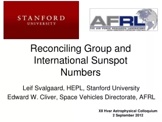
Reconciling Group and International Sunspot Numbers Leif Svalgaard, HEPL, Stanford University Edward W. Cliver, Space Vehicles Directorate, AFRL NSO Workshop 26 30 April 2012
Sunspot Number • Primary time series in solar & solar-terrestrial physics: • applications to dynamo studies and climate change • Two SSN series that vary widely during the 19th Century
The Sunspot Number(s) • Wolf Number = kW (10*G + S) • G = number of groups • S = number of spots • Group Number = 12 kGG Rudolf Wolf (1816-1893) Observed 1849-1893 Ken Schatten
The Ratio Group/Zurich SSN has Two Significant Discontinuities At ~1946 (after Max Waldmeier took over) and at ~1885
Corroborating Indications of the ‘Waldmeier Discontinuity’ ~1946 • SSN for Given Sunspot Area increased 21% • SSN for Given Ca II K-line index up 19% • SSN for Given Diurnal Variation of Day-side Geomagnetic Field increased by 20% • Ionospheric Critical Frequency foF2 depends strongly on solar activity. The slope of the correlation changed 20% between sunspot cycle 17 and 18
Sunspot Areas vs. Rz The relationship between SSN and sunspot area [SA, Balmaceda et al., 2009] is not linear, but can be made linear raising SA to the power of 0.732. Pink squares show the ratios for SA exceeding 1000 micro-hemispheres Clear change in the relationship around 1945
What caused the Waldmeier Discontinuity?
At some point during the 1940s the Zürich observers began to weight sunspots in their count Weights [from 1 to 5] were assigned according to the size of a spot. Here is an example where the three spots present were counted as 9, inflating the sunspot number by 18% [(3*10+9)/(3*10+3)=1.18] Waldmeier claimed that the weighting scheme dates from 1882. However, Wolfer (1907) explicitly states that he counts spots without regard to size
Removing the discontinuity in ~1946, by multiplying Rz before 1946 by 1.20, yields Leaving one significant discrepancy ~1885
Independent • Group Sunspot Number Determination • Includes all major observers from 1825-1900 • Based on group counts (scaled to Wolfer who • observed from 1876-1928)
1876-1893 Wolfer Group SSN Count Wolf Group SSN Count Wolfer reported 65% more groups than Wolf
Group SSN Count (Wolfer) 15 Observers: Wolfer, Broger, Madrid, Leppig, Moncalie, Pastorff, Quimby, Schmidt, Schwabe, Shea, Spoerer, Tacchini, Weber, Winckler, Wolf ------ = Ri/12 No significant systematic difference between Ri & Rg
Confirmed by a technique based on geomagnetic data: It has been known since 1852 that the daily range of geomagnetic activity varies with the SSN (Wolf & Gautier) Morning Evening
The Diurnal Variation of the Declination for Low, Medium, and High Solar Activity
The Diurnal Range rY is a very good proxy for the Solar Flux at 10.7 cm F10.7, in turn, is highly correlated with the SSN 16
The most recent long-term solar reconstructions based on 10Be data from ice cores is generally consistent with our result Steinhilber et al. (2010)
Removing the discontinuity in ~1885 by multiplying Rg by 1.47, yields There is still some ‘fine structure’, but only two adjustments remove most of the disagreement and the evidence for a recent grand maximum
Conclusions • Group SSN is flawed and should be abandoned • No evidence for Grand Maximum from ~1945-1995
Text to accompany slides: • Title & Affiliations • 2) Self-explanatory • 3) Before ~1880, Group sunspot numbers (GSNs) are often ~30-50% lower than the • Wolf (also called International or Zurich SSNs). • 4) Rudolf Wolf proposed the above formula for the International sunspot number (ISN). • Thus a group consisting of a single spot would have an ISN of 11. Because Wolf did • not count relatively small spots, all subsequent observers (who do count such spots) • have a “K” or an observer factor of about 0.6, to bring their counts down to that of • Wolf. Also shown is a picture of a young Ken Schatten, who developed the GSN with • Doug Hoyt. For the group count only individual groups are counted. Conceptually this • seems simpler because, after all, who cannot see a group? In practice, particularly as • one goes back in time as smaller telescopes and different techniques were used (e.g., • that of Wolf), observers differ on group counts and thus K factors are required for the • GSN as well. The 12 is used to normalize the SN to the ISN. It indicates that on • average, a group has two sunspots. • 5) The ratio of monthly GSN to ISN since 1850. There are two significant discontinuities • in the time series of this ratio that we will examine, in turn. The most recent occurred in • ~1945 when Waldmeier took over the responsibility for making the ISN from Brunner.
6) Several lines of evidence corroborate the discontinuity. We will discuss the first of these. 7) Self-explanatory. 8) Self-explanatory. 9) This finding by Leif was a real surprise because the ISN was universally thought to be calculated using the formula from the earlier slide. In fact, since Waldmeier the individual spots have been given weights and a test conducted by Leif and one of the observers at Locarno, the standard station for making the ISN, showed the magnitude of the difference to be slightly less than 20%. The difference from 20% is possibly due to a difference in the definition of groups instituted by Waldmeier at the same time. 10) Self-explanatory. 11) During the last several months, Leif has made an independent, straight-forward, determination of the GSN time series. The procedure was to use group counts for all significant observers from Schwabe to 1900 and to scale their counts to Wolfer. This procedure differs from that of Hoyt and Schatten who used Greenwich instead of Wolfer as the standard observer. Leif found that the Greenwich counts were inhomogeneous during the 19th century, a result that was recently verified independently by Jose Vaquero.
12) This slide shows the standard procedure for determining the relationship (K-factor relative to Wolfer’s 1.0) for all observers. Wolf’s K-factor in this determination of the GSN is 1.65. 13) The net result for all 15 observers. The dashed black line is the ISN or Ri divided by 12, the normalization factor between the GSN and ISN time series and the thin blue line is the composite result for the 15 observers. Thus there appears to be no significant or systematic differences between the ISN time series and the GSN time series as determined by Leif. Hoyt and Schatten’s method is complex and not terribly well described but one clear indication of a problem is the fact that they had nearly equal K-factors for Wolf & Schwabe relative to the Greenwich data. 14) The above result receives independent corroboration from an independent SSN-calibration techniques based on geomagnetic data, specifically the regular variation due to ionization of the dayside ionosphere by solar EUVg radiation. The current vortices that are thus established, have measurable magnetic fields at the ground that have been Measured for nearly 300 years.
15) This slide shows data from Prague, for recent times on top, and ~150 years ago on the bottom. The individual panels show the variation of one of the components of the B-field (in this case the declination) over the course of a 24-hour day for each of the 12 months of the year. In the top , the blue line represents the relatively weak variation at solar minimum relative to the black line for solar maximum. The red and pink lines to the right show the averages for the periods considered. The data at the bottom shows that the same characteristic curves were observed ~150 years ago. The arrow on the bottom right indicates that it is not the 24-hour range that is of interest buy rather the total variation during the sunlit hours. 16) The range thus measured for the eastward component of the magnetic field (rY) is highly correlated with the 10-cm radio flux which, in turn, is highly correlated with the SSN, and which can thus be used to calculate the SSN for earlier times when measurements of rY are available. 17) This slide puts the geomagnetic-based reconstruction of the ISN on the same time scale as that of the re-derived GSN (now multiplied by 13 to give the ISN), the GSN of Hoyt and Schatten, and the ISN. As can be seen, the GSN time series is too low before ~1885. 18) The result from the previous slide is further support by a recent reconstruction of solar wind B based on 10Be-data from ice cores which is generally consistent with the IDV-based reconstruction of Svalgaard & Cliver (2010).
19) Here we show that it is necessary to increase the GSN by 47% before ~1885 to bring it into agreement with the other time series. This is not entirely an academic exercise because extending the series of group counts initiated by Leif may be the most straight- forward way of extending the ISN back in time. 20) Self-explanatory with the caveat to first conclusion that the GSN may be a useful stepping stone to extending the ISN further back in time.