Download
1 / 22
220 likes | 298 Views
On-Line Decision Problems with Exponentially Many Experts. Richard M. Karp Hoffman Fest September 19-20, 2014. On-Line Decision Problem.

E N D
On-Line Decision Problems with Exponentially Many Experts Richard M. Karp Hoffman Fest September 19-20, 2014
On-Line Decision Problem A game between an adversary and a chooser. At each of T steps the adversary secretly designates a subset of a fixed set A of n possible actions. The designated actions are called winning and the others are called losing. • The chooser, knowing the winning actions at all preceding steps, chooses an action. • The set of winning actions at the current step is then revealed to the chooser. • The chooser’s goal: Minimize regret, the number of times he chooses a losing action, minus mine(number of losses of action e). • Any deterministic policy for the chooser can be made to lose at every step.
Randomized On-line Algorithms with Proven Regret Bounds • {W(t,e), L(t,e))}: Number of {wins, losses} for action e in first t steps. • Multiplicative Update Algorithm: Choose a small positive epsilon. At each step t+1, assign a weight (1-epsilon}(L(t-1,e))to each action e. Draw an action from a distribution in which the probability of an action is proportional to its weight. • Kalai-Vempala Algorithm: at each step t+1, assign each action e the score W(t,e) - R(t+1,e) where R(t+1,e) is drawn by the chooser from an exponential distribution with mean 1/epsilon. Choose the action argmaxeW(t,e) – R(t+1,e)
Bounds on Regret For the multiplicative weight update algorithm and Kalai-Vempala algorithm the expected regret after step t is at most epsilon mint L(t,e) +O(log(n)/epsilon where n is the number of possible actions.
Examples • The actions may be: paths through a network, multicommodity flows, packings of a knapsack, truth assignments, stock levels in an inventory system, spanning trees, minimum spanning trees, perfect bipartite matchings, transversals in a bipartite graph, bases in a matroid etc. • How to implement the Kalai-Vempala algorithm when the number of possible actions is exponentially large?
Coping with Exponentially Many Actions • Approach: Find a compact representation that enables counting the number of winning actions at any prior step, sampling uniformly at random from the set of winning actions at that step , and testing whether a given action is winning at that step. • Implement the Kalai-Vempala algorithm using these primitives.
Ideal Case • WIN(t) Set of winning actions at step t. • Ideal case: It is possible to count the elements of WIN(t), sample uniformly from WIN(t) and test membership in WIN(t). • Sets for which the ideal case holds: source-sink paths respecting a deadline, feasible solutions to a provisioning problem, feasible solutions to a knapsack problem, spanning trees, minimum spanning trees, satisfying assignments to a boolean formula described by a BDD.
Nearly Ideal Case • Approximate counting can be done. The nearly ideal case applies to perfect matchings in a bipartite graph, integer multicommodity flows, satisfying assignments to a DNF Boolean formula and bases of a transversal matroid.
Example: The On-Line Path Selection Problem • The setting: A graph G, a source a and sink z, where a is different from z, and a positive integer deadline d. • The actions are the paths from a to z in G. • At each step t the adversary assigns positive integer costs to the edges. A path is winning if the sum of the costs of its edges is less than or equal to d.
A Compact Representation • A pair (c,u), where c is a nonnegative integer and u is a vertex, is good at step t if there is a path of cost c from a to u and a path of cost <=d-c from u to z. • In the graph of winning paths H the vertex set is the set of good pairs plus the pair (d,z) and there is an edge from (c,u) to (c’,v) if c’ –c is the cost of edge (u,v) and from (c,u) to (d,z) if the cost of the edge (u,t) is less than or equal to d-c. • The winning paths are the paths in H from (0,a) to (d,z).
Constructing the Graph H • By breadth-first search forward from (0,a) and backward from (d,z) find the set of winning pairs. • Counting: Examining the pairs (c,u) in H in decreasing order of c, compute L(c,u), the number of paths in H from (c,u) to (d,z). L(0,a) is the number of winning paths. • Sampling: Impose an arbitrary linear ordering on the edges out of each pair in H. This induces a linear ordering on the winning paths. For any N, one can quickly find the Nth path in this ordering.
A Provisioning Problem • Each day, the adversary secretly specifies a vector d = (d(1),d(2),…,d(m)) of demands for m perishable goods and the chooser chooses supply levels e(1),e(2),…,e(m) summing to C. The action (e(1), e(2),…,e(m)) is winning if e(i) >= d(i) for all i. Easy exercise: count the winning choices and sample uniformly at random from the set of winning choices.
Naïve Algorithm for the Ideal Case • At step t+1 explicitly compute W(t,e) and W(t,e) - R(t+1,e) for all e, and choose argmaxeW(t,e) – R(t+1,e). Here W(t,e) = W(t-1,e) + 1 if e is a winning action at time t, and W(t-1,e) otherwise. This is expensive of time and especially of storage.
Thinning • Choose a small positive parameter p • At each step, compute a thinned winning set in which each winning action occurs independently with probability p • Estimate each W(t,e) by V(t,e)/pwhere V(t,e) is the number of thinned winning sets containing e at the first t steps. Execute the naïve algorithm using these estimates.
Intersection Trick Winning sets: WIN(1), WIN(2),…,WIN(T) In many cases, the intersection of k winning sets has a compact representation supporting counting, uniform sampling and membership testing. One can estimate the fraction of winning sets containing action e up to time t by picking random k-tuples of prior winning sets and estimating the frequency with which the k-fold intersection contains action e.
A Thought Experiment A thought experiment: given an urn filled with balls of many different colors, find all balls that occur with frequency at least 1/r, where r is positive integer. Solution: Repeat as long as possible: discard a set of r balls of distinct colors. At the end of this process, fewer than r colors remain, and every color of frequency >1/r in the original urn isamong them.
Finding Frequent Actions with Limited Storage WIN(i) = set of winning actions at time i. Action e is (t,r)-frequent if W(t,e) > 1/r (|WIN(1)| + … + |WIN(t)|). Problem: for t=1,2,…,T find the (t,r)-frequent actions. These are candidates for argmaxe (W(t,e) –R(t+1,e)). Actions that are not (t,r)-frequent can often be eliminated.
A Streaming Algorithm • Process the successive sets WIN(1), WIN(2), …, WIN(T) action by action. • Create sets S(1),S(2), each of cardinality at most r and containing occurrences of distinct actions. • Place each action in turn in the first set that can accept it.
Streaming Algorithm (continued) • A set S(j) is incomplete if it contains fewer than r distinct actions. For each such action, the algorithm keeps a count of the number of incomplete sets containing the action. • Lemma: At any point, the number of actions occurring in incomplete sets is less than r. • Lemma: If action e is (t,r)-frequent then, after the processing of WIN(1), WIN(2),…,WIN(t), action e occurs in at least one incomplete set.
Estimating the Frequencies of Actions • Goal: for each action e, estimate the number of complete sets containing e. • Associate with each complete set S(j) a consensus set C(j) as follows: C(1) = S(1) for j=2,3,… if e is in both S(j) and C(j-1) then e is in C(j) pair the remaining elements of S(j) one-to-one with the remaining elements of C(j-1). Place one action from each pair into C(j), choosing the element from S(j) with probability (j-1)/j, and the element from C(j-1) with probability 1/j.
Estimating the Frequencies of Actions (continued) • Theorem: The probability that action e lies in C(j) is exactly number of occurrences of e in the sets S(1), S(2),…,S(j), divided by j. The construction of the consensus sets C(t) is randomized. By maintaining several consensus sets for each set S(t) one can estimate the number of occurrences of e in the sets S(1),S(2),…,S(t). Combining this with the construction of the (t,r)-frequent actions one can reliably estimate argmaxeW(t,e) –R(t+1,e) for all t.
Acknowledgement This is ongoing joint work with EvdokiaNikolova of UT Austin. The further work will focus on algorithms for the non-ideal case, in which counting and sampling can only be done approximately, and the non-binary case, in which an action receives a score ate each step, rather than merely winning or losing.