Download
1 / 47
470 likes | 539 Views
Regional Automaton. CS 5270 Lecture 7. Today…. Bisimulation – an equivalence relation Rationals into integers Regional equivalence Representation of regions Zones DBMs Graph interpretations. Back to last 10 slides of lect 6…. Both the set of states and actions are infinite. TTS.

E N D
Regional Automaton CS 5270Lecture 7 Lecture 8
Today…. • Bisimulation – an equivalence relation • Rationals into integers • Regional equivalence • Representation of regions • Zones • DBMs • Graph interpretations Lecture 8
Back to last 10 slides of lect 6… Both the set of states and actions are infinite. TTS Semantics TSTTS Finite set of actions but infinite set of states. TATTS Regions RTS Both states and actions are finite sets. Lecture 8
Rationals to integers…. • TTS = (S, S0, Act, X, I, !) • Let m1/ n1, m2 / n2,…, mk / nk be all the (irreducible) rationals that appear in the transitions. Let K be the LCM of {n1, n2,.., nk}. • Transform a constraint of the form x · m/n into x · (m/n) £ K etc. • Let TTS’ be the resulting timed transitions system. Then s is reachable in TTS iff it is reachable in TTS’. • TTS’ has only integer-valued constants in the guards! Lecture 8
An example x 1.2 ; y y < 2.3 x < 2.1 y > 2 a b 2.1 = 21/10 1.2 = 12/10 2 = 20/10 2.3 = 23/10 Lecture 8
An example x 12 ; y y < 23 x < 21 y > 20 a b Reachability properties will be preserved… Lecture 8
The Equivalence based on Regions. • TA = (S, S0, Act, ) • tµS£S , a bisimulation of finite index. • (s, V) t (s’, V’) iff • s = s’ • V Reg V’ ( V and V’ belong to the same region). Lecture 8
Regional Equivalence – V Reg V’ • X = {x1, x2, …, xn}, the set of clock variables. • V, V’ ---- Two clock valuations. • V : X R • V’ : X R • V Reg V’ ? • r 2R. • b r c , the largest integer less than or equal to r. (the integral part of r). • b 2.8 c = 2 • bc = 3 • r 2R • fr( r ) , the fractional part of r. • r = b r c + fr(r) Lecture 8
Regional Equivalence – V Reg V’ • X = {x1, x2, …, xn}, the set of clock variables. • V, V’ ---- Two clock valuations. • V : X R • V’ : X R • V Reg V’ ? • cx = MAX{ c | “x REL c” is a clock constraint appearing in some guard or invariant} • x REL c ----- x ≤ c x ≥ c x < c x > c • We are assuming all constants mentioned in the guards are integers. Lecture 8
An example x 12 ; y y < 23 x < 21 y > 20 a b Cx = ? Cy = ? Lecture 8
Regional Equivalence – V Reg V’ • X = {x1, x2, …, xn}, the set of clock variables. • V, V’ ---- Two clock valuations. • V Reg V’ iff (i) For every x, either • b V(x) c > cx and b V’(x) c > cx OR • V(x) · cx and V’(x) cx. Further, V(x) = V’(x) and fr(V(x)) = 0 iff fr(V’(x)) = 0 (ii) Suppose V(x) · cx and V(y) · cy. Then fr(V(x)) · fr(V(y)) iff fr(V’(x)) · fr(V’(y)). Lecture 8
An example x 12 ; y y < 23 x < 21 y > 20 a b V’(x) = 87 V’(y) = 21.8 V(x) = 22 V(y) = 21.6 Lecture 8
An example x 12 ; y y < 23 x < 21 y > 20 a b V’(x) = 24 V’(y) = 21.6 V(x) = 22 V(y) = 21.6 Lecture 8
An example x 12 ; y y < 23 x < 21 y > 20 a b V’(x) = 20.8 V’(y) = 21.9 V(x) = 20.4 V(y) = 21.6 Lecture 8
An example x 12 ; y y < 23 x < 21 y > 20 a b V’(x) = 20.8 V’(y) = 21.9 V(x) = 20.4 V(y) = 21.6 Lecture 8
An example x 12 ; y y < 23 x < 21 y > 20 a b V’(x) = 20.8 V’(y) = 21 V(x) = 20.4 V(y) = 21 Lecture 8
Example X = {x, y} cx = 2 cy = 1 {(0, 1)} is a region. {(x, y) | 0 < x = y < 1} is a region. 28 regions. Lecture 8
Regional Equivalence • Reg is an equivalence relation of finite index! – (see Katoen handout) • Each equivalence class of Reg is called a region. • There are only a finite number of regions. Lecture 8
The Equivalence based on Regions. • TA = (SV, svin, Act, ) • tµSV SVa bisimulation of finite index. • (s, V) t (s’, V’) iff • s = s’ • V Reg V’ ( V and V’ belong to the same region). Lecture 8
The Quotienting • One member of a clock region satisfies a clock constraint iff all members of the clock region satisfy the clock constraint. • This can be used to compute the t -quotient of TA, called the regional transition system. Lecture 8
The Reductions. Both the set of states and actions are infinite. TTS Semantics TSTTS Finite set of actions but infinite set of states. TATTS Regions RTS Both states and actions are finite sets. Lecture 8
Time Abstraction • TTS = (S, S0, Act, X, I, !) s 2 S • TSTTS = (SV, svin, Act [R, )) • TATTS = (SV, svin, Act, ) where : • (s, V) (s’, V’) iff there exists such that • (s, V) ) (s, V+) in TS and • (s, V+) ) (s’, V’) in TS. a a Lecture 8
The Region Automaton • TATTS = (SV, svin, Act, ) • (s, V) (s’, V’) iff s = s’ and V and V’ belong to the same clock region. • [(s, V)] --------- (s, [V]). • RTS = (SRV, srVin, Act, ) • SRV = {(s, [V]) | (s, V) in SV } • srVin = (sin, [Vzero]) = (sin, {Vzero}) • (s, [V]) (s’, [V’]) iff for some V1 in [V] and some V1’ in [V’] it is the case that in TATTS, (s, V1) (s’, V1’) a a Lecture 8
Example: TTS Lecture 8
The Representation of Regions • For each clock x specify one formula of the form: • c x < c + 1 where c is in {0, 1, …., cx -1} OR c = cx OR x > cx • For each clock pair specify a constraint of the form x – y = 0 or x – y < k or y –x < k for a suitable k in case x cx and y cy. Lecture 8
Example: The Regional Transition System. Only the reachable states have been shown.
The Regional Construction • Given a timed transition system, its (finite!) regional transition system can be computed effectively. • Hence one can effectively solve the reachability problem (and other verification problems) concerning timed transition systems. • This is the mathematical basis for the verification tools for timed transition systems and timed automata. Lecture 8
Zones • A more compact representation. • Of equivalence classes of valuations. • Can be efficiently represented as Difference Bounded Matrices (edge weighted directed graphs). • DBMs admit a canonical representation. • DBMs can be manipulated efficiently. Lecture 8
Why not regions? • The number of regions can be very large: • Exponential in the number of clocks AND in the size of the maximal constants appearing in the clock constraints. • Practical verification becomes infeasible. Lecture 8
An Example y x Lecture 8
0-dimensional regions: 12 y x Lecture 8
1-dimensional regions: 23 y x Lecture 8
2-dimensional regions: 12 y x Lecture 8
Total number of regions: 47 y x Lecture 8
One Zone: (2 ≤ x ≤ 5) (2 ≤ y ≤ 4) y x Lecture 8
Termination • To ensure termination: • Remove constraints of the form x < m , x ≤ m, x – y < m and x – y ≤ m if m > Cx. • Replace x > m and x m with x > Cx if m > Cx. • Replace y – x > m and y – x m with y –x > Cx and y – x Cx when m > Cx. Lecture 8
Zone operations • We need to compute D. • Given D1 and D2, we need to compute D1 D2. • Given D and D’ we need to be able to check if D is a subset of D’. • We must be able check if D is empty. Lecture 8
Zone representation. • A zone can be represented as a DBM: • Difference Bounded Matrix. • Invent a new clock variable x0 (which will always be 0). • All basic constraints will be of the form xi – xj < m or xi – xj≤ m where m is an integer (positive or negative). Lecture 8
Zone Representation • x2 < 3 becomes x2 – x0 < 3. • X5 7 becomes x0 – x5≤ -7. • X2 – x5 > 8 becomes x5 –x2 < -8. Lecture 8
The Matrix Representation. x0 x1 x2 . . . xj xn x0 x1 x2 . .xi . xn xi – xj ≤ 2 (2, ≤) Lecture 8
The Matrix Representation. x0 x1 x2 . . . xj xn x0 x1 x2 . .xi . xn xi – xj< 2 (2, <) Lecture 8
The Matrix Representation. x0 x1 x2 . . . x3 (3, <) x0 x1 x2 . .x3 . ∞ (-4, <) (10, <) (2, <) (5, <) (2, <) Lecture 8
The Graph Representation (k, ≤) (k, <) x y x y y – x ≤ k y – x < k Lecture 8
The Graph Representation 10 X1 X2 -4 2 3 2 X3 X0 5 Lecture 8
Closed Representations • Two different zones (DBMs) can represent the same set of valuations. • (y – x ≤ 3, x = 2, y = 4) (y –x = 2, x =2, y = 4) • A zone is closed if no constraint can be strengthened without reducing the set of associated valuations. • Two closed zones are equivalent iff they are identical. • So it is good to get closed zones. Lecture 8
Closed Zones. • Take the graph of the zone. • Remove all redundant edges. • The edge from x to y with weight k is redundant if there is a path from x to y whose weight is less than or equal to k. • Using a shortest path algorithm, the closed zone version can be computed in O(n3) time. Lecture 8
Closed Zones • If D is closed then D is a subset of D’ iff for every constraint x – y ≤ m’ in D’ there is a constraint x – y ≤ m in D with m ≤ m’. • If D is closed then D is non-empty iff there are no negative weight cycles in the graph. • The other operations can also be performed on the graphs efficiently. Lecture 8